Simulating and Prototyping
a Formula SAE Race Car Suspension System
Mark Holveck ’01
Rodolphe Poussot ’00
Harris Yong ’00
Submitted to the Department of Mechanical and Aerospace Engineering, Princeton University in partial fulfillment of the requirements of Undergraduate Independent Work.
Progress Report
January 5, 2000
Advisor: Prof. Seymour Bogdonoff
Reader: Prof. Jeremy Kasdin
MAE 439
Special formatting is described on page
The authors would like to give special thanks to:
The Mechanical and Aerospace Engineering Department at Princeton University, for encouraging the Formula SAE project and for their financial support.
Jim Arentz at Penske Racing Shocks, for the prompt design of suitable adjustable dampers.
Professor Seymour Bogdonoff at Princeton University, for his advice for the direction of the Formula SAE team, his focus on the larger picture of car design and pointing out the necessity of sensitivity analysis.
Scott Badenoch at Delphi Chassis, for his insights on suspension design of Formula SAE cars.
Steve Dalstrom at TrueChoice Motorsports, for assisting us with hardware selection.
Lawrence Gunn at Reynard Motorsport, for providing us with free versions of the Reynard Kinematics suspension geometry software.
AJ Jones and Chris Joehenning at Goodyear Tire & Rubber, for comprehensive tire performance data.
Professor Jeremy Kasdin at Princeton University, for keeping in constant contact with the authors, keeping us on schedule.
Arron Melvin at Princeton University for assisting in all aspects of design and parts sourcing and for acting as an active member of the Princeton Formula SAE Vehicle Control Division.
Glenn Northey at Princeton University, for manufacturing and design advice.
Rodney Sparks at California State University, Sacramento, for the suggestions on suspension kinematics, packaging and hardware.
Christopher Yanchar at General Motors Vehicle Dynamics, for sharing his experiences and knowledge gained by being a member of the University of Minnesota Formula SAE experience team.
Princeton University MAE Undergraduate Independent Work
Although this paper focuses on the suspension system of the Princeton Formula SAE car, some areas are written to describe the consideration given to the other components and systems that govern or place limitations on the suspension design. This paper is meant to be a progress report for the Princeton Formula SAE car suspension system and outlines the work performed by the Princeton Formula SAE Vehicle Division, which is responsible for the suspension, wheel, tire, brake and steering systems of the Formula SAE car.
Because of the wealth of information accrued over the past several months, it is impossible to reference every fact, especially those acquired from non-standard literature, such as electronic resources, contact with professionals, etc. An effort has been made, however, to give credit to sources providing unique information. The more well known and generic suspension design criteria and definitions cited have their references given on page
*, along with sources that the authors consulted but whose works are not quoted directly.No oversize or color pages are contained in this report, although there are high resolution graphics and tables.
Acknowledgements
*Prefaces
*Princeton University MAE Undergraduate Independent Work
*References
*Formatting
*Table of Contents
*List of Figures
*List of Tables
*List of Symbols
*Abstract
*Introduction
*Defining a Suspension System
*Philosophy and Goals in the Context of Formula SAE
*Design Preliminaries
*Design Overview
*Table of Main Parameters
*Design Procedure
*Basic Assumptions and Estimates
*Preliminary Design Choices
*Suspension Kinematics
*Basic Geometric Parameters
*Derived Front View Parameters
*Derived Side View Parameters
*Steering Considerations
*Designing with Reynard Kinematics
*Suspension Dynamics
*Parameters for Understanding Suspension Dynamics
*Analyzing and Designing Suspension Dynamics Parametrically Using Microsoft Excel
*Vehicle Dynamics Simulation Using CarSim Educational
*Suspension Loads
*Manufacturing details
*Progress Summary and Future Work
*Summary
*Future Work
*References
*Appendices
*Definitions (Suspension Kinematics)
*Definitions (Suspension Dynamics)
*Vehicle Dynamics Calculations Spreadsheet
*Penske 8750 Damper Dyno Plots
*A-Arm Dimensions
*Front Suspension Load Calculations
*Rear Suspension Load Calculations
*Goodyear Tire Curves
*Purchased Parts, Suppliers and Prices for Fall 1999
*
Figure 1. The University of Leeds Formula SAE car. (Formula SAE 1999 brochure)
Figure 2. Princeton Fomrula SAE car frame.
Figure 3. Side view of the frame identifying supsension mounting locations.
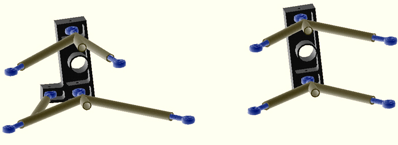
Figure 4. Drawings of the left rear suspension (left) and the left front suspension (right), looking out from the inside of the car. The front of the vehicle is to the right.
Figure 5. Front view of the left front suspension on a prototypical section of the frame.
Figure 6. An A-arm. (Milliken)
Figure 7. Double A-arm suspension system. (Milliken)
Figure 8. Non-independent suspension system.
Figure 9. An inboard suspension system on a CART car. (World Wide Web)
Figure 10. Tire camber curves.
Figure 11. Intended front suspension toe curve.
Figure 12. Camber gain from caster (when the front wheels are steered).
Figure 13. Front view swing arm and instant center concept. (Milliken)
Figure 14. The effect of front view swing arm length on camber gain. (Milliken)
Figure 15. The effect of front view instant center height on tire scrub. (Milliken)
Figure 16. Defining the instant centers. (Milliken)
Figure 17. Defining the roll center. (Milliken)
Figure 18. The jacking effect.
Figure 19. Front suspension roll center height as a function of roll.
Figure 20. Rear suspension roll center height as a function of roll.
Figure 21. Anti-dive geometry.
Figure 22. Anti-squat geometry. (Milliken)
Figure 23. Anti-lift geometry. (Milliken)
Figure 24. One possible orientation for rear steer Ackermann steering. (Milliken)
Figure 25. A-arm suspension system. Rightmost image shows an ungrounded track rod. (Milliken)
Figure 26. "Initial" sheet in Reynard Kinematics.
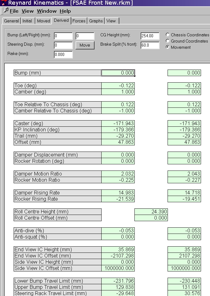
Figure 27. "Derived" sheet in Reynard Kinematics. The caster and kingpin inclination are wrong by 180 degrees (program bug), and the sing of the trail is reversed. "Anti-" values are not calculated correctly by Reynard Kinematics for the Princeton Formula SAE car’s suspension geometry.
Figure 28. "Moved" sheet in Reynard Kinematics.
Figure 29. View of front suspension system in Reynard Kinematics. This image is a view from outside the front left corner of the car.
Figure 30. View of rear suspension system in Reynard Kinematics. This image is a view from outside the front left corner of the car.
Figure 31. Lateral load transfer as a function of CG height. (Lopez)
Figure 32. The roll axis as defined by the roll centers, and related parameters. (Milliken)
Figure 33. Front left upright under 1.5G right turn cornering and 1.2G braking.
Figure 34. Suspension uprights. Left image is rear upright. Right image is front upright.
Figure 35. Basic tire/wheel orientations. (Milliken)
Figure 36. Tie rod too short causes toe changes (bump steer). (Milliken)
Figure 37. Tie rod in the wrong vertical location causes toe changes (bump steer). (Milliken)
Figure 38. Suspension and steering geometry. (Milliken)
Figure 39. Spreadsheet showing the calculation of vehicle dynamics parameters.
Figure 40. Front damper dyno plot.
Figure 41. Rear damper dyno plot.
Figure 42. Front suspension A-arm dimensions.
Figure 43. Rear suspension A-arm dimensions.
Figure 44. Front suspension load calculations.
Figure 45. Rear suspension load calculations.
Figure 46. Tire curves showing lateral force generated as a function of various parameters for a 19.5x7.5x10 Goodyear tire.
Table 1. Main parameters of the Princeton Formula SAE suspension system.
Table 2. A possible procedure for designing a Formula SAE race car suspension system.
Table 3. Table summarizing effects when parameters that deviate from the design intent.
Table 4. Summary of suspension member loads.
Table 5. Table of Fall 1999 purchases.
List of SymbolsThis list contains symbols used in the main textual body of the paper.
|
Symbol |
Meaning |
|
CG |
Center of gravity |
|
deg |
Degree (angular) |
|
ft |
Foot |
|
FVSA |
Front view swing arm |
|
G |
Acceleration equivalent to the acceleration of gravity on earth |
|
Hz |
Hertz |
|
IC |
Instant center |
|
in |
Inch |
|
lb |
Pound of force |
|
LLTD |
Lateral load transfer distribution |
|
mm |
Millimeter |
|
RC |
Roll center |
|
SVSA |
Side view swing arm |
The primary goal of a suspension system in the context of a Formula SAE vehicle is to provide an interface between the tires and the car body that allows the race car to provide a high level of road handling in a predictable fashion under all expected accelerations and forces. Although this goal is superficially simple, the selection of parameters to achieve the ideal suspension system is the result of evaluating and weighing numerous competing minor objectives, many of which require iterative calculations and educated predictions of values that cannot be measured until an entire vehicle is constructed. This paper summarizes the basic suspension parameters that need to be considered in race car suspension design, not only by defining the parameters but also by considering the effects of one parameter on the others. By analyzing parameters and objectives in terms of suspension kinematics, suspension dynamics, and suspension loads, as is done in this paper, the art of suspension design becomes more manageable. These design considerations have resulted in the construction of one front and one rear suspension system prototype, both unequal length A-arm designs featuring outboard spring/damper systems, manufactured for Princeton University’s first Formula SAE car. This paper also highlights the role of computer simulation and parametric tools in the choice of suspension parameters. It should serve as a summary of suspension basics in the context of a vehicle control system, as a list of lessons learned from design and also as a guideline for further exploration in future design iterations.
A generic suspension system consists of three groups of components: suspension links or control arms (the solid members that define the structure of the suspension system), springs that absorb the energy from road inputs that would otherwise be transmitted directly to the vehicle body, and dampers (sometimes less appropriately referred to as shock absorbers) that control wheel and body motion by dissipating energy stored in the springs by means of heat.
For a race car, the role of the suspension system is to manage forces produced in accelerations from propulsion, braking, cornering and ground input. Providing a comfortable ride to the car’s occupants—an important consideration for passenger cars—is of less importance in a race car as long as the driver is not affected so severely that his or her physical ability in controlling the car is compromised. It is important to remember that despite the analysis of the suspension system detailed in this paper, all longitudinal and lateral accelerations generated by a vehicle are governed by the tires and their contact patches on the ground. Thus, behind all the calculations is the goal of managing the tire’s contact patch, and the ideal race car suspension system is one that can transfer the forces needed to generate car accelerations to the ground in a manner that is most manageable for the tires on the ground. This is done by finding the most appropriate compromise among many objectives, including strength, low weight, geometry/kinematics (the path the wheels take relative to the car, as defined by the suspension components, when subjected to the acceleration inputs) and dynamics (the control of car body and wheel motion).
For the Princeton Formula SAE suspension design, a left hand coordinate system is used for each end (front and rear) of the vehicle, centered along the centerline of the car. Each coordinate system is located centrally between the wheels of each axle, and at the center of the bottom tube of the frame. Positive X points rearward, positive Y points to the left front wheel of the car, and positive Z points away from the ground. The choice of a left hand coordinate system is because the software used, Reynard Kinematics, utilizes this coordinate convention. The kinematics and geometry design is done fully in SI units (with lengths in millimeters), but the dynamics and manufacturing details are specified in the US Customary System for the ease of manufacturing and for dealing with suppliers.
Suspension dynamic considerations can be classified into four main dynamic modes of vehicle motion: roll (vehicle rotation about the longitudinal X axis resulting from cornering forces), pitch (vehicle rotation about the Y axis resulting from longitudinal accelerations due to drive torque and braking), heave (uniform rectilinear motion along the Z axis of each tire), and warp (the non-uniform variant of heave). These modes will be discussed in more detail in the Dynamics section of the report. A not so obvious consideration is the ground clearance of the car as it limits the amount of motion the car may safely and predictably attain under dynamic loading.
Philosophy and Goals in the Context of Formula SAE
Formula SAE is an intercollegiate competition, sponsored by the Society of Automotive Engineers and by other organizations and corporations in which about 100 colleges worldwide participate. At the center of its competition concept is the construction of an open wheel formula racer that excels not only on paper but also by performing well in dynamic events.
Because a Formula SAE car entrant represents a prototype for the nonprofessional weekend autocross driver, the suspension system on the car must thus be manufactured at a reasonable cost and feature reliability in addition to its dynamic performance. In the spirit of the competition, the design and manufacturing of the suspension system detailed in this paper reflects the four philosophical emphases embraced by the Princeton University Formula SAE team for its first car, namely simplicity, adjustability, upgradability and integration (with other components). In addition, reliability is also a major concern for a first Formula SAE car as the completion of the events would give the insight required to rethink and reconsider the major decisions that were made for the first iteration.
To place the suspension design in context of a Formula SAE car, a picture of a Formula SAE car is provided as Figure 1, and an image of the computer designed Princeton Formula SAE frame is shown as Figure 2. Figure 3 shows the locations of the front and rear suspensions. It is important also to keep in mind the environment in which Formula SAE cars are expected to perform. The dynamic events are held at a stadium parking lot that is relatively smooth and level asphalt except for unavoidable wear and tear. The vehicle is expected to compete in the following types of dynamic events: acceleration event, autocross (tight course to evaluate the car’s overall abilities), endurance race, and skidpad (circle track to evaluate the car’s steady state cornering ability). Wet weather performance is not a serious concern for Formula SAE cars.
Before getting into the details, (numbers and physics) of suspension design, the authors would like to describe the basic layout of Princeton Formula SAE car’s first suspension system. The proposed suspension layout consists of fully independent, unequal length double A-arms at all four vehicle corners with a short knuckle, or in-wheel design. Outboard coil springs over dampers provide the necessary springing and damping, and an anti-roll bar will be incorporated into the front suspension, with a provision for a bar at the rear suspension if testing deems it necessary. A more detailed summary of the suspension system, including numerical values is given in Table 1.
Drawings of the Princeton Formula SAE suspension systems are shown as Figure 4. The left image shows the control arms and upright for the rear system, and the right image shows the same items for the front system Both are for the left side of the car. A front view picture of the front suspension a few days prior to completion is shown in Figure 5.
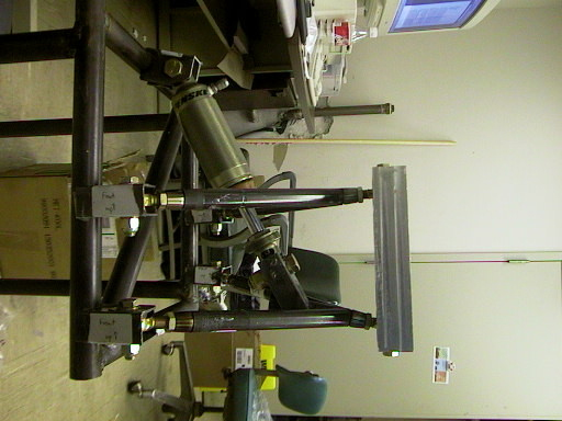
Figure 5. Front view of the left front suspension on a prototypical section of the frame.
|
Front |
Rear |
Units |
|
|
Overall Vehicle |
|||
|
CG height |
12 |
12 |
in |
|
Sprung mass |
225 |
275 |
lb |
|
Sprung mass distribution |
45 |
55 |
% |
|
Tire size |
18x7.5x10 |
18x7.5x10 |
- |
|
Track |
1200 |
1200 |
mm |
|
Unsprung mass |
45 |
45 |
lb |
|
Wheel diameter |
10 |
10 |
in |
|
Wheel width |
8 |
8 |
in |
|
Kinematics |
|||
|
Anti-dive |
12 |
- |
% |
|
Anti-lift |
- |
5 |
% |
|
Anti-squat |
- |
12 |
% |
|
Brake bias |
60 |
40 |
% |
|
Caster |
8.1 |
6 |
deg |
|
Ground clearance |
37.2 |
37.2 |
mm |
|
Kingpin inclination |
0 |
0 |
deg |
|
Roll center height |
24.4 |
52.9 |
mm |
|
Static Camber |
-1 |
-1.5 |
deg |
|
Static Toe-In |
-0.12 |
0.12 |
deg |
|
Dynamics |
|||
|
Damper rate (compression) |
14.3 |
29.3 |
lb/(in/sec) |
|
Damper rate (rebound) |
42.1 |
86.3 |
lb/(in/sec) |
|
Motion ratio |
0.489 |
0.383 |
- |
|
Ride frequency |
2 |
2.2 |
Hz |
|
Ride rate |
46 |
68 |
lb/in |
|
Roll gradient |
2 |
2 |
deg/G |
|
Spring rate |
200 |
491 |
lb/in |
|
Materials |
|||
|
Upright |
aluminum |
aluminum |
|
|
Control arms |
4130 steel |
4130 steel |
|
|
Bracketry |
4130 steel |
4130 steel |
Table 1. Main parameters of the Princeton Formula SAE suspension system.
The design procedure used by the authors are similar to that specified in Woods and Jawads’ guidelines but has undergone significant revision to produce an expanded version shown as Table 2.
|
# |
Procedure |
Category |
Comments |
|
1a |
Establish vehicle parameters (size, weight, power, etc.) |
Preliminary |
The range of values for basic vehicle parameters such as size and power to weight ratio are defined, explicitly or indirectly, by the rules and regulations of the Formula SAE competition. |
|
1b |
Specify basic suspension type and geometric layout. |
Preliminary |
|
|
1c |
Specify springing medium layout (inboard/outboard) |
Preliminary |
|
|
2 |
Specify suspension kinematics details. |
Kinematics |
The specification of suspension geometry and kinematics, because of the details and iterative nature, takes considerable time despite only occupying one entry in this table. More details are given later. |
|
3a |
Estimate corner weights (sprung and unsprung). |
Dynamics |
|
|
3b |
Specify ride frequencies and ride frequency ratio. |
Dynamics |
The ride frequencies may need to be modified according to the expected wheel displacements calculated in step 3e. |
|
3c |
Derive ride, suspension and spring rates. |
Dynamics |
|
|
3d |
Derive initial roll rates without anti-roll bars. |
Dynamics |
|
|
3e |
Evaluate wheel displacement at maximum accelerative loads. |
Dynamics |
Repeat steps 3b-3e as necessary. |
|
3f |
Calculate lateral load transfer distribution (LLTD) between the front and rear axles without anti-roll bars. |
Dynamics |
|
|
3g |
Specify anti-roll bars to produce desired roll rates and LLTD. |
Dynamics |
Because Microsoft Excel can be used to determine derived values, anti-roll bar requirements need not be explicitly solved for. Instead, one can iteratively edit anti-roll bar dimensions until the desired LLTD is obtained. |
|
3h |
Specify damper rates. |
Dynamics |
Damper values can be specified as early in the procedure as after the derivation of spring rates. |
|
4 |
Select sizing and material of control arms and mounting hardware |
Loads |
Sizing and material selection can be made a higher priority in the design procedure if experience suggests that these parameters are attainable without compromising the dynamic factors significantly. |
Table 2. A possible procedure for designing a Formula SAE race car suspension system.
Basic Assumptions and Estimates
Some assumptions and estimates need to be made clear at this point. Their implications on suspension design will be covered later.
Overall laden vehicle mass with driver:
590 lb. This estimate is based on the tabulated data of the most recent Formula SAE entries.Static front/rear sprung mass (weight) distribution:
45% front, 55% rear (also denoted 45/55). These numbers mean that the fore/aft location of the center of gravity of the sprung mass is slightly to the rear of the midpoint between the front and rear tires. The sprung mass is the mass that is supported by the springs of the suspension system, which excludes items such as tires, wheels, control arms for most suspension systems, etc.Unsprung mass:
23 lb per corner. This is the estimate of the mass that is not supported by the suspension system and includes, if applicable, for each vehicle corner, a wheel, a tire, the control arms, the upright/hub assembly, a driveshaft, a brake rotor, a caliper and mounting hardware. The rear unsprung mass does not include a brake rotor and caliper because an inboard brake design is expected, but it includes a driveshaft for torque transmission, which the front suspension does not include.Center of gravity (CG) height:
12 in. This is an estimate based on data from other Formula SAE entries and is on the conservative (high) side. A conservative value is assumed because the CG height plays a significant role in all the dynamic calculations, and a high CG height will underestimate the capabilities of the car.Rigid frame:
Despite the careful analysis performed by the Body Division, it is natural for any vehicle frame to deflect under loading. In the preliminary design of a suspension system, however, the frame is generally taken to be infinitely rigid such that calculations and estimates can be performed. At the time of publishing this report, the Princeton Formula SAE Body Division is estimating a front to rear bending rigidity of 490 ft-lb/deg and a side to side bending rigidity of 760 ft-lb/deg, values which are perhaps several factors lower than the numbers needed to produce a rigid race car.Highest steady state acceleration values:
Although many suspension characteristics determine the capabilities of the car, estimates of acceleration magnitudes are necessary to determine certain suspension parameters. The acceleration values suggested here are the result of discussions with other schools, published data in literature as well as test data from the Goodyear Tire & Rubber Company. Braking deceleration: 1.2 G Cornering lateral acceleration: 1.5 G. Forward acceleration: < 1 G.Ground clearance:
From discussion with other teams, a ground clearance of about 50 mm is sufficient to handle all accelerations for commonly used spring rates. Most calculations and design procedures detailed in this report are based on the ground to frame distance of 50 mm. However, because the Body division is using one inch outer diameter tubing, the actual ground clearance (before having the frame scrape the ground) is closer to 37.3 mm. Calculations detailed later show that even this reduced clearance is sufficient to handle the highest steady state acceleration under the design conditions.,Wheelbase:
The wheelbase (distance between the front and tire contact patches) was set at 1700 mm early in the design process with other Princeton Formula SAE team members. This is just slightly below the majority of the competition as it was a goal to produce a somewhat smaller and more maneuverable car.Track Widths:
Both the front and track widths (distance between the left and right tire contact patches) were specified, in collaboration with other Princeton Formula SAE team members, to be 1200 mm . The track widths can be easily changed later in the design process when all the hardware (hubs, brake rotors and hats) are specified because the track widths have no effect on the frame dimensions. Again, track widths of 1200 mm are slightly below the majority of the competition to create a relatively nimble car at the sacrifice of slightly increased load transfer.Preliminary Design Choices (Steps 1a-1c)
As mentioned earlier, the authors have chosen a double A-arm design for the first iteration of Princeton University’s Formula SAE car suspension. This choice was primarily based on considerations of suspension geometry or kinematics—the subject of how the wheels and other unsprung masses of the vehicle are connected to the sprung vehicle body. The suspension kinematics determines not only how the sprung and unsprung masses move relative to each other but also how the forces are transmitted among them. .
Before justifying the double A-arm choice, it is necessary to consider the primary suspension layout variations. The first major categorical division among suspension types is independent vs. non-independent. As its name suggests, independent suspensions are ones whose wheel paths are entirely decoupled.. A non-independent suspension system has its left wheel and right wheel rigidly connected such that the motion of one wheel affects the other in a geometrically constrained manner. Independent suspensions have several advantages, one of which is that, compared to non-independent suspension, they provide an inherently higher roll stiffness relative to the vertical spring rate.
Since there are six degrees of freedom for a moving object (three translational axes and three rotational axes), and because the wheels should have a single (curvilinear), well defined path at all times, it is clear that independent suspensions should have only one degree of freedom, or five degrees of restraint. For non-independent suspensions where two wheels are coupled together, there are two degrees of freedom (the two wheels can move in the same or in opposing directions), so there are four degrees of restraint. Each of these degrees of restraints will require one suspension control arm or link in compression and tension. Alternatively, a control arm can also be placed in bending and torsion so that it can provide more than a single degree of restraint.
Because non-independent suspensions require one fewer degree of restraint than independent suspensions, they are often simpler to manufacture, by rigidly connecting the left and right wheels together. On the other hand, the coupling of the wheels is often undesirable, especially on imperfect roads, because each wheel cannot be controlled independently. This means that wheel travel paths on non-independent suspension systems are greatly compromised. Thus, non-independent suspensions were ruled out early in the design procedure for the Princeton Formula SAE car.
There are many specific layouts among independent suspensions, but they can all be classified based on the number of links it uses to provide the five degrees of restraint. Common designs are considered here. For instance, the simple trailing arm uses one link to provide all five restraints by placing the arm in not only axial loading but also bending and torsion. Variations include the semi-trailing arm and the swing axle. The McPherson strut uses four links (the sliding strut acting as two links, the lower control arm consisting of two links and a tie rod). Finally, among the common designs, the double A-arm and some other more elaborate designs use a link for each degree of restraint, thus allowing each link to be placed in pure tension or compression. In this way, the double A-arm is structurally superior to designs that use fewer links. Furthermore, it offers flexibility in the choice of suspension kinematic details and parameters. It is no wonder that the double A-arm design is the design of choice for most race cars. It also offers easy packaging, especially for formula style race cars where the body is relatively narrow compared to the track widths. The drawback is that it requires a larger number of components (five links including the tie rod).
Another preliminary design choice consideration is the location of the spring and damper. There are two basic configurations, inboard and outboard. An outboard design is one in which the spring and damper are located in the area of the control arms, with one end near the wheel and one end near the body, and where the control arms or hub assembly directly applies forces to the spring and damper. The outboard design is used on all street vehicles. An inboard design is where the at least one additional axially loaded member is used to translate the force(s) from the wheel to the spring and damper, which are usually located within the main body of the car. Figure 9 shows a picture of an inboard system.
The current trend for formula style cars is the inboard design. However, the authors have chosen an outboard design for the first Princeton Formula SAE race car. In high speed motorsports, an inboard system is necessary to decrease aerodynamic drag and manage lift, neither of which is a consideration for the Formula SAE competition due to the lower vehicle speeds. The inboard system, although reducing space in the control arm area, crowds the cockpit area of a vehicle and increases the suspension design complexity due to the added link(s) needed to transfer wheel forces to inboard springs and dampers. However, the inboard system does have an unquestionable advantage in compactness. This is because the spring and damper can be designed smaller because they can be placed in an orientation that takes only axial loading, whereas an outboard spring and damper will almost always take some off-axis loading. Although more compact, the weight savings of an inboard design’s compactness is debatable because additional hardware (e.g., bellcrank, rocker) is needed. What this additional hardware allows is further adjustability. For example, a rocker can be designed to offer wheel rates that are progressive (non-linear and stiffer springing with wheel deflection). Very complex designs, such as T anti-roll bars and a third spring that activates only on dive or squat (body pitching) are also possible.
In summary, the inboard system is akin to the independent suspension layout in that it offers added adjustability and the possibility of reduced weight at the expense of some complexity. In this case, however, the authors feel that the increased adjustability is beyond the needs of a first Formula SAE car, and that the other benefits of the inboard system do not justify its implementation considering its added complexity.
Another preliminary design choice is the wheel diameter. The major tire suppliers for Formula SAE, namely Goodyear and Hoosier, offers tires for mounting on 10 inch and 13 inch wheel diameters. The trend for Formula SAE teams is to use 13 inch wheel diameters because this gives more room within the wheel where suspension and brake components can be packaged. However, preliminary calculations showed that, even with 10 inch wheels, satisfactory suspension kinematics could be obtained. The final go ahead of the 10 inch wheel diameter was given after the authors received confirmation that brake rotors and calipers were available for the 10 inch wheel diameter. With a 10 inch wheel diameter, unsprung weight can be reduced slightly, reducing the moment of inertia of the wheel bearing, wheel and tire combination. The wheel diameter also affects the size and shape of the contact patches of the tires. More information has not been readily available from the tire manufacturers, and despite the increasing use of 13 inch diameter wheels, there have been numerous cars that have utilized the 10 inch diameter wheels well.
Suspension Kinematics (Step 2)
The authors feel that the best way of describing the design of the Princeton Formula SAE suspension kinematics is by stepping through the kinematic parameters, and how they affect each other. The parameters are not ordered alphabetically but in a way so that one who is unfamiliar with suspension design can read through the next few pages in sequence and understand new ideas as they are introduced. After the discussion on kinematic effects is a section on how the Princeton Formula SAE suspension was designed using computer software. Because of the large number of suspension terms and jargon, an appendix of formal definitions of the basic geometric parameters is on page
*. The body of the report will only discuss the effects and implications of the various parameters and not its definitions. Readers not familiar with the parameters listed below may find it helpful to refer to the Appendix.Camber is a main factor affecting the lateral force road holding ability of tires, meaning that the camber characteristics of a suspension system constitute one of the most important considerations within suspension kinematics. Because the control arms of a suspension system are fixed in length, the camber will change as a function of wheel travel. As a vehicle rolls to the outside of a corner when turning, camber on the outside tire will grow in the positive direction unless the suspension kinematics build in negative camber under bump conditions. A good suspension system will maintain optimal camber under a variety of cornering loads. Most tires operate best between 0° and –3° of camber, and a tire’s ability to generate lateral (cornering) forces under various conditions is shown in the Appendix on page
*. The change in camber with wheel travel is known as camber gain. For small angles of body roll as seen in a formula style car, the approximate camber change needed to keep the tires flat on the road is given by Equation 1, where d is the wheel displacement (positive for bump), and t is the track width of the end of the vehicle under consideration (1200 mm for the Princeton Formula SAE car).![]()
Equation 1.
To offset the positive camber induced by body roll, a suspension can provide negative camber by building in sufficient camber gain or by starting with the tires cambered slightly negative and building in relatively less camber gain. Although the latter method means that the camber can only be optimized for a small range of wheel displacements, it has its merits. First, building in sufficient camber gain to offset the camber loss as given in Equation 1 means that the camber will change significantly under braking and acceleration when the camber change is not needed, resulting in less predictable traction management. Starting out with static negative camber also has benefits in reducing the rolling resistance of the tires, thereby reducing the power needed to accelerate the vehicle and to maintain a constant speed. Lastly, it may be difficult to build in the exact camber gain when other objectives are considered.
For the Princeton Formula SAE car, the static negative camber is set at –1° for the front tires and –1.5° for the rear tires and can be varied by adjusting the rod ends between the control arms and the uprights. The camber curves (camber with respect to bump) for the front and rear suspension system of the Princeton Formula SAE car are given as Figure 10, and the camber Equation 1 is plotted together for comparison.
Figure 10. Tire camber curves.
Note that the rear suspension’s camber curve is less than optimal (does not gain sufficient negative camber) for wheel displacements greater than about 38 mm of travel. At lower magnitudes of wheel displacement, the camber is overly negative (due to the initial static negative camber). The front suspension’s camber curve is less aggressive (less camber change with wheel displacement) because caster is used to generate camber for the front suspension.
Although tire wear is at a minimum when there is zero toe (tires are parallel and point straight ahead), there are conditions where some toe is beneficial. In general, toe-in results in increased straight-line stability, while toe-out quickens transitional behavior. If any toe is incorporated into the rear tires, it is almost always toe-in because this reduces the tendency for the rear end of the car to become loose during cornering. There is not as strict a rule of thumb for toe on the front tires. The static toe values are not as important for suspension design, and they can be altered by adjusting rod ends on the tie rods. The front tires are tentatively set to have about –0.12° of toe (toe-out) and the rear toe is specified to be 0.12° (toe-in).
The Princeton Formula SAE car has a toe curve that goes toward toe-in on bump for the front tires. This helps to increase stability in braking and point the front outside tire in the steered direction during a turn. Currently there is no bump steer built into the rear suspension. The authors are considering building in toe-in on rebound such that there is increased stability upon braking and the rear wheels rebound. However, large changes in rear toe can lead to a less predictable car. Figure 11 shows the intended front toe curves for the Princeton Formula SAE car. The toe change is minimal with respect to bump and rebound, although there is some curvature at high rebound. This should not pose a problem as dynamic calculations show that wheel travel should not be much more than 35 mm in both bump and rebound. Furthermore, the vertical scale shown in Figure 11 is very magnified. Because there is no bump steer for the rear suspension, the toe curve is flat at its static toe in of 0.12° and is not shown here.
The trail provides a torque that recenters the wheels when they are steered The mechanical trail of the Princeton Formula SAE car is 29.3 mm for the front suspension, and 17.0 mm for the rear suspension, which is in the correct range according to other Formula SAE teams for sufficient self-centering of the front wheels.
A positive caster creates the mechanical trail needed to recenter the steered front wheels. In addition, positive caster generates negative camber on the outside tire when the wheel is steered, and positive camber on the inside tire, both of which offset the camber loss due to body roll. Another effect of caster is that it raises the steered outside wheel relative to the car, so the outside front corner of the car drops relative to the rest of the vehicle. This creates a diagonal load transfer away from the heavily loaded front tire to the less loaded inside rear tire and creates an oversteering effect while contributing to more responsive turn-in behavior.
Because of the positive effects of camber gain and diagonal weight transfer effects of positive caster, the Princeton Formula SAE car incorporates approximately 8° of positive caster on the front suspension system. Typical street cars have between 3° to 6° of positive caster. The camber gain from caster alone is shown in Figure 12 and helps to explain why less camber gain is built into the control arms for the front suspension system.
Because 8° of caster generates significant mechanical trail, the ball joints for the front of the Princeton Formula SAE car have been translated rearward. That is, instead of moving the upper ball joint back and the lower ball joint forward an equal distance from the wheel vertical centerline, the lower ball joints are 5.9 mm in front of the wheel centerline, and the rear ball joints are 14.1 mm behind the wheel centerline.
Ideally, for rear wheel drive cars, the scrub radius is slightly positive. This gives a good feel of the road through to the driver via the steering wheel. If the front left tire hits a bump, a counterclockwise torque is generated about the steering axis and tugs the steering wheel in the same direction. However, excessive scrub radius can make the car very unstable on a bumpy road, requiring constant driver input to hold the steering wheel steady. In front wheel drive cars, the scrub radius has to be negative to combat the effects of torque steer. Since no Formula SAE car is driven by the front wheels, the effects of a negative scrub radius will not be discussed here.
Usually, if a kingpin inclination exists, the upper ball joint is farther inboard than the lower ball joint, so only the kingpin inclination in this orientation is considered. The kingpin is usually inclined due to packaging and scrub radius considerations; with the upper ball joint inboard of the lower ball joint, the scrub radius can be reduced to a manageable level. Kingpin inclination also has the effect of raising the steered front end of the vehicle, adding to the weight that the front tires have to carry. This in itself is not necessarily an undesirable effect, but the other effect of kingpin inclination—always generating undesirable positive camber for the steered wheels—means that it is the goal of a suspension designer to minimize kingpin inclination.
The Princeton University Formula SAE car is designed to have no lateral kingpin inclination at all to minimize poor camber and the decreased predictability of having weight transferred to the front wheels when they are steered. The use of zero kingpin inclination is often precluded because of the goal of reducing the scrub radius, but with wheels that have sufficient positive offset (the hub mounting face close to the outside of the wheel), zero kingpin inclination can be attained.
One way of reducing kingpin inclination is to package both upper and lower ball joints within the wheel (also known as a short knuckle, or in-wheel design) so that the scrub radius is reduced without the need to angle to the steering axis. The short knuckle may increase the loads on some control arm members due to reduced spread between the upper and lower ball joints, but it has benefits of being able to change wheel or tire size without widening the track and increasing the spindle length and scrub radius after the design is completed.
The basic geometric parameters have now been discussed. Derived geometric parameters are explained below, together with their consequences on vehicle dynamics.
Front View Swing Arm (FVSA) and Instant Centers (IC)
The paths taken by the wheels of a complex suspension system can be found by replacing all the control arms of a corner of a vehicle with virtual swing arms, one in the front view and one in the side view. In the front view, the swing arm extends from the wheel center above the centerline of the tire to a point called an instant center (IC), as shown in Figure 13.

Figure 13. Front view swing arm and instant center concept. (Milliken)
The wheel path in this view is then defined by rotating the wheel about the instant center, keeping the swing arm at the same angle to the wheel as it was in the static position. Figure 14 shows how the front view swing arm length directly affects the camber gain.

Figure 14. The effect of front view swing arm length on camber gain. (Milliken)
The camber gain is then defined by Equation 2 for small angles.
![]()
Equation 2.
The front view swing arm length at the static ride height position is about 2115 mm for the front suspension and 935 mm for the rear suspension, explaining why the camber gain curve for the front suspension (as shown in Figure 10) is not as steep as the rear suspension’s.
In the front view of the swing arm, the instant center height governs the lateral movement of the tire during bump and rebound. Figure 15 shows that, with the instant center on the ground, there is minimum movement of the tire relative to the ground (scrub).

Figure 15. The effect of front view instant center height on tire scrub. (Milliken)
With the instant center below the ground, the tire moves toward the body on bump; the opposite is true if the instant center is above the ground. Thus, in the interests of tire wear and tracking on bumpy roads, the instant center should be on the ground, but this can severely limit the choices available in suspension kinematic design. In most cases, scrub is not very significant, so instant center height in the front view is not a major consideration.
The instant center is determined, in double A-arm suspensions, by finding the point at which the lower and upper control arms would converge if their lengths were extended. See Figure 16. Lastly, the instant center is called "instant" because its location varies with wheel travel on most designs. To get a larger picture the suspension kinematics, the change in instant location with respect to wheel travel should be considered.

Figure 16. Defining the instant centers. (Milliken)
Roll Centers (RC) and Roll Axis
The roll centers (one for the front suspension and one for the rear suspension) are among the most important parameters in performance car suspension design. Whereas important parameters such as mass of the car and the center of gravity cannot be changed from a suspension designer’s point of view, the roll centers can be. The front roll center is the point around which the front of the vehicle rolls under the force imparted by a lateral acceleration. The rear roll center is the same geometric point for the rear suspension. Joining the front and rear roll centers creates a line called the roll axis, which is the line about which the entire vehicle rolls. Before describing how the roll centers are determined, it is important to note that, because the roll centers are defined using the front view instant centers, the roll center also moves, changing in height from the ground and also shifting left and right across the car.
The roll centers are basically determined from the front view instant centers and the vehicle track widths. To generate the roll center position for a suspension, a line is drawn from the contact patch of the left tire to its instant center, and another line from the contact patch of the right tire to its instant center. The roll center is where the two constructed lines cross. For a symmetric suspension on a car that is not experiencing roll, the roll center’s lateral location will be at the centerline of the car. On most designs, when a car drops in ride height, the roll centers will also drop. When a car rolls, the roll center will usually move laterally and vertically.

Figure 17. Defining the roll center. (Milliken)
The roll centers are important because they determine the force coupling point between the unsprung and sprung masses. For example, if the roll centers were at the same height as the center of gravity and remained there with bump and rebound, the car would not roll at all during cornering because the moment arm between the center of gravity and the roll centers would be nonexistent. The lower the roll center, the larger this rolling moment becomes.
The other primary effect of roll center location—jacking—is not as obvious. If the roll center is anywhere other than on the ground plane, any lateral force generated by a tire will create a moment about the front view instant center. This will either jack up the body of the car (move the car body up if the roll center is above ground) or jack down the body of the car (if the roll center is below ground). Figure 18 shows a jacking up effect of a high roll center. In the dynamics section of this paper, it will become evident how the roll center heights directly determine the load transfer distribution between the front and rear axles.

Figure 18. The jacking effect.
Summary of Front View Suspension Kinematics
The analysis of the front view suspension kinematics is now complete. From the roll center discussion alone, it can be seen that there are already competing objectives. To create a car that does not roll, the roll centers have to be as high as the center of gravity. However, this means a severe jacking up effect. If the roll center were placed on the ground plane, jacking would not be a problem, but the large rolling moment would mean building in a large amount of suspension travel and good camber gain characteristics over this travel to make ensure that the tires are well positioned relative to the ground for maximum lateral grip. Large amounts of body roll also has negative effects in that the weight transfer rate is lowered, causing a delayed reaction of the car body when given a steering input. The common and modern way of approaching these conflicting objectives is to maintain a relatively large rolling moment by using low roll centers but stiffer springs or anti-roll bars to reduce the amount of body roll. Yet the suspension cannot be overly stiff or else it cannot deal with road disturbances properly. The difference in heights of the front and rear roll centers also affect the dynamics of the vehicle and will be treated in the Suspension Dynamics section of the paper.
The Princeton University Formula SAE car has its roll centers at 24.4 mm above ground at the front and 52.9 mm above ground at the rear. Throughout all expected roll and heave behavior, the rear roll center remains above the front roll center. This intent of the designers is due to a dynamics consideration addressed later. Although some cars have begun to place their roll centers below the ground plane, the Princeton University Formula SAE car has its roll centers above the ground to retain the traditional feel of jacking up the body instead of jacking down the body. Because the roll centers move down with body roll, starting with relatively higher roll centers means that the roll centers will not cross the ground plane under light lateral accelerations. Crossing the ground plane is regarded as a destabilizing effect by some because the jacking forces reverse directions. Under all circumstances, the roll centers should not go above the center of gravity height because that would cause the vehicle to roll into a turn like a bicycle, and if this happened under high lateral accelerations, the car would immediately lose stability. See Figures 19 and 20 to see how the roll centers move with roll and bump; with 31.5 mm of bump on one side and 31.5 mm of bump on the other, the front roll center drops to about 127 mm below ground, while the rear roll center is at about 7 mm below ground. Thus, the front roll center is much more sensitive to roll. The dynamic results of this are discussed later.
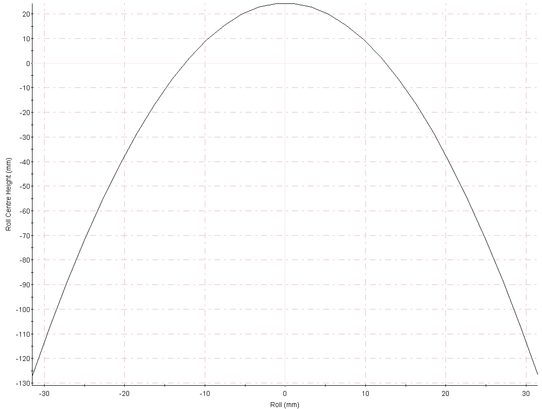
Figure 19. Front suspension roll center height as a function of roll.
. 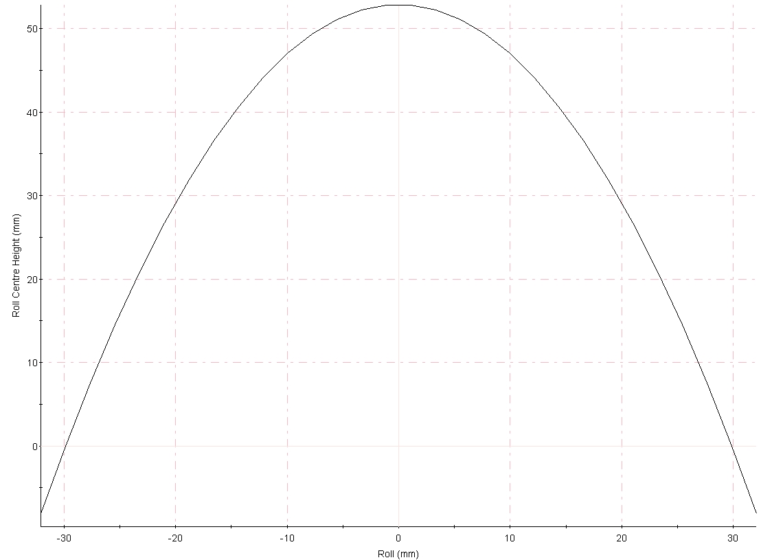
Figure 20. Rear suspension roll center height as a function of roll.
Side View Swing Arm (SVSA) and Instant Centers
The side view geometry is determined by where the upper and lower A-arms converge if they were larger in the front to rear direction. From the side view of the car, most suspension designs allow the wheel to travel straight up and down. Applying the swing arm and instant center concept, this means that the side view swing arm length is infinite, with the side view instant center located infinitely far away. Analogous to the arguments made for the location of the front view instant center, the location of the side view instant center will determine how the wheelbase changes with bump and rebound. The effects of the side view swing arms and instant centers are not as pronounced, except for "anti" characteristics, described below.
Just as the front view roll centers describe indirectly the force coupling between the horizontal and vertical factors, "anti" effects describe longitudinal and vertical force coupling. Because a car is not front-rear symmetric, "anti" effects are often harder to visualize than front view effects. The "anti" effects considered for the Princeton Formula SAE car include front anti-dive, rear anti-squat and rear anti-lift. Note that these "anti" effects do not change the steady state loads on the tires, but they do affect the pitch attitude of the car.
When a car decelerates from foot brake application or engine braking, the front wheels carry more load than they carried statically even in the absence of pitching. The dynamics of this are considered later. By moving the side view instant center upward, some of the force that would be resisted by the springs can be resisted by the control arms. This means that the car dives less under braking. Figure 21 shows the derivation of anti-dive amounts for a front suspension with outboard brakes. Notice that, for anti-dive, the side view instant center has to be behind the center of the wheel and above the ground. The anti-dive is calculated as a percentage, as shown in Equation 3.
![]()
Equation 3.
The percentage indicates the amount of load that is taken up by the control arms instead of the springs. CG is the height of the center of gravity (12 in), and l is the wheelbase (1700 mm). The brake bias is assumed to be 60% front and 40% rear for this calculation.
Although a side view instant center is really only well defined if the control arms are not parallel in the side view, the Princeton University Formula SAE car does use control arms that are parallel in the side view so that the caster does not change with bump and rebound. For the front suspension, the both the upper and lower control arms are tilted at about 2° upward. This side view geometry does mean that the front wheel travels upward and forward in bump, thereby increasing the wheelbase very slightly. The front wheels traveling forward under bump is often avoided in street cars because the ride can become harsher. However, the authors feel that the anti-dive requirement outweighs the desirability of ride quality. Also, this method of incorporating anti-dive essentially eliminates the change in caster during body pitching, so the steering feel is more consistent with braking load. The 2° tilt gives an effective SVSA height to SVSA length ratio of 0.035. Assuming that the front wheels do 60% of the braking, the front suspension incorporates about 12% anti-dive. Anti-dive is limited usually to a 25% maximum because some dive is necessary for the driver to gauge braking force, and because the control arms should not take too much of the braking force or else suspension component binding, or worse, failure, could result.
Rear anti-squat refers to the side view control arm design to resist the rear of the car squatting under forward acceleration. Rear anti-lift refers to the design that counteracts the rear of the vehicle rising under deceleration.
Whereas front anti-dive means that suspension travels forward during bump, both rear anti-squat and rear anti-lift require the side view instant center to be placed ahead of the wheel center and above the ground, so the rear wheels move rearward during bump. Thus, rear anti-squat and rear anti-lift do not conflict with the goals of ride quality.
Because the Princeton Formula SAE car will use inboard rear brakes, the control arms do not provide brake reaction torque. Therefore, the effective SVSA height is not measured from the ground up but from the wheel center up, as shown in Figure 22.

Figure 22. Anti-squat geometry. (Milliken)

Figure 23. Anti-lift geometry. (Milliken)
The control arms are again tilted, but it is the front of the control arms that are raised, and at about 1.25° . Using Equations 4 and 5 and a brake bias of 60% front, 40% rear, the side view geometry of the rear suspension results in 5% rear anti-lift and 12% rear anti-squat.
Equation 4.
![]()
Equation 5.
A brief discussion of steering parameters not mentioned above is given here. The authors found it necessary to do some preliminary research on steering parameters as they govern aspects of suspension design
Tie Rod/Track Rod/Lateral Link Location/Compliance Steer
All wheels require one link/suspension member to provide proper lateral location. On a steered front wheel, a tie rod, connected to the steering rack, is used to provide lateral and directional control of the wheel. In the rear, the link that provides lateral resistance is often called a lateral link. The term track rod is sometimes used in place of tie rod and lateral link. Above, some information has been provided on the importance of the track rod lengths and orientation with the effects on bump steer. In addition, under high lateral loads, the suspension members deflect, leading to compliance steer, where asymmetric forces cause changes in geometry that in turn steer the wheels. Compliance steer is especially evident on street cars that use rubber bushings. Because compliance steer is often non-linear and difficult to model, suspension and steering components should be designed such that any compliance steer creates an understeer effect. In other words, front suspension members should behave in a way to cause toe-out, and rear suspension members should cause toe-in. This way, the heavily loaded outside tires will point, due to compliance understeer, in directions that increase the turning radius. When the contact patch of the heavily loaded outside wheel provides a lateral force on the suspension pointing toward the car body, the compliance is such to generate positive camber. To generate compliance understeer for the front wheels (toe-out), the tie rods should be located in the upper rear of the wheel or the lower left of the wheel, as shown in Figure 38 in the Appendix. For both of these locations, when the outside wheels are forced to positive camber, and the tie rods, in resisting the positive camber, will provide a torque about the steering axis that causes toe-out. Given the design of the frame around the front suspension area, the authors have chosen to go with a rear steer design, with the track rods placed above the center of the wheels.
For the rear wheels, the track rods should be in the unshaded areas of Figure 38 in the Appendix to produce toe-in of the outside wheel under lateral loading (again compliance understeer). This location of the track rod also adds to the loads imparted on the lower front control arm, and packaging is difficult because the rear shock is also mounted on the same arm. The authors plan to stay with the design of an ungrounded track rod. This means that, instead of providing lateral location of the wheel by creating a member joining the rear upright and the frame, the lateral link starts from the upright but terminates at the control arm, as shown in the rightmost image of Figure 25. This reduces an attachment point at the frame but adds slightly to the loading on the control arm member to which the track rod attaches.
The authors have designed full Ackermann steering for the Princeton Formula SAE car. The reasons for this will be discussed in the Spring 2000 paper when steering system details are covered. The use of full Ackermann steering is mentioned here because it affects the design of the front uprights.
At this design stage, the brake considerations mainly relate to packaging. Rotors with a diameter of 7.5" and suitable calipers have been sourced, and preliminary calculations show that these small rotors will provide adequate heat capacity and require brake line pressures and pedal forces that are manageable in magnitude.
Designing with Reynard Kinematics
This section outlines how the basic kinematic design can be accomplished using Reynard Kinematics. The advantages of software design is evident with Reynard Kinematics because the method is truly parametric. First, all control arm points are in the rectangular XYZ coordinate system on a Microsoft Excel spreadsheet, together with basic suspension type and definitions. These points are read in by Reynard Kinematics and displayed on a sheet called Initial. Figure 26 shows the locations of the relevant data points (the front suspension sheet is shown). Toe, camber, tire diameter, wheelbase and rake are entered in separately. Because an outboard suspension does not have a pushrod to actuate springs and dampers, the values here are arbitrary. The rocker locations have been set to simulate the spring and dampers being fixed at the frame end and to move with the lower control arms.
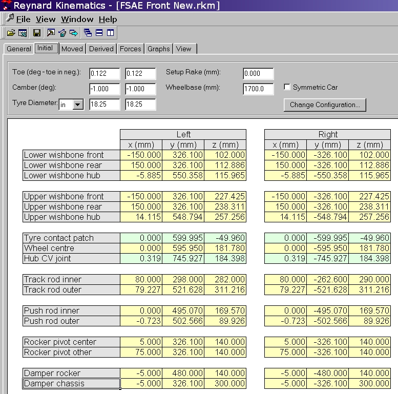
Figure 26. "Initial" sheet in Reynard Kinematics.
The initial values now affect all other calculations, such as the Derived sheet for the front suspension as shown in Figure 27. Virtually all of the important parameters such as toe, camber, caster, kingpin inclination, trail, roll center locations, etc., are shown. This sheet also allows one to put in bump values for each wheel, as well as steering input to see how these factors affect suspension kinematics. Rake, the forward and rearward pitching of the car, is not used. Instant center locations are also given, and they can be used to calculate "anti" effects. Because the definitions of "anti" effects with Reynard Kinematics are not documented, the authors chose to derive their own "anti" calculations for the time being.
A Moved sheet (Figure 28 shows the front suspension Moved sheet) details how the coordinates of each point moves with bump, steering and rake and can be used to determine why derived suspension parameters change the way they do.
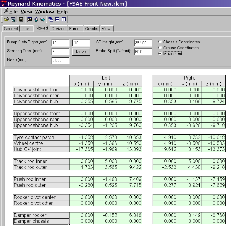
Figure 28. "Moved" sheet in Reynard Kinematics.
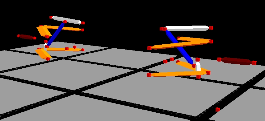
The View sheet allows a designer to see the created suspension, using different colors for different components. The view orientation can also be changed, and steering and bump can be input for motion visualization. A view of the front suspension is shown in Figure 29, oriented such that the front of the vehicle is in the lower left corner of the image. The very top member shows the current thinking for tie rod location (rear steer above the wheel centerline, as discussed earlier). The two extensions off to the side of the suspension are not part of the front suspension system. The small, light colored vertical links near the end of the lower control arms are pushrods that are not used for the Princeton Formula SAE Suspension System.
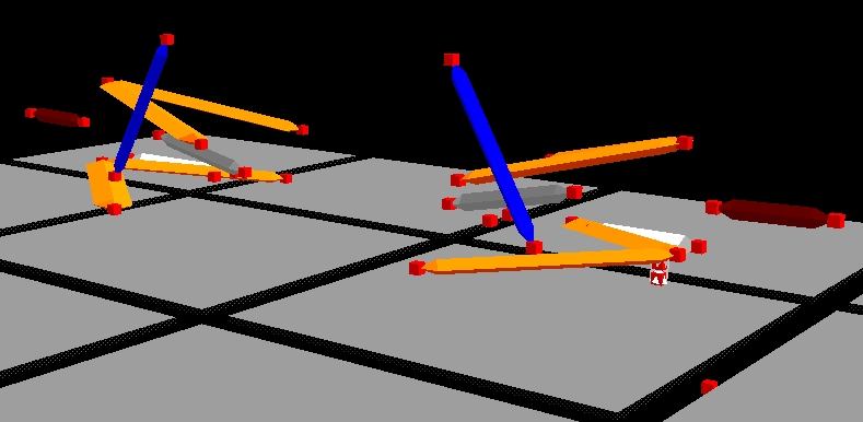
A rear suspension view is shown as Figure 30. The link that is between the upper and lower control arms is an approximation for the driveshafts. The angle of the control arms is farther from being parallel to the ground, partly the result of roll center and camber gain specifications. It may be difficult to see in Figure 30, but the lower control arms are mounted on the frame slightly outboard of the upper control arm locations. The view also shows the springs and dampers mounted on the lower control arm.
A powerful capability of Reynard Kinematics is its ability to graph all the suspension parameters with respect to bump, steer and roll. This is what was used to generate the various curves derived earlier, and the plots can be output to Microsoft Excel for further manipulation.
Suspension Dynamics (Steps #3a-3h)
Whereas suspension kinematics defines the wheel path and types of forces each suspension member experiences, suspension dynamics determines the magnitudes of these forces and thus the accelerations and amount of movement of both the unsprung and sprung masses.
As in the preceding section on Suspension Kinematics, the discussion on Suspension Dynamics will begin with the implications of certain parameters. As with suspension kinematics, formal definitions of these terms are given in the Appendix, on page
*. Because of the nature of suspension dynamics, a step by step consideration of the determination of various rates and loads will illustrate the design process more effectively.Parameters for Understanding Suspension Dynamics
To generate any lateral force, a slip angle must be present. This is why slip angle is a very important parameter in tire data, along with camber angle and normal load.
With static toe-in or toe-out, the tires are forced to travel straight ahead, while the wheels are pointed slightly in or out, respectively. This generates a slip angle. Thus, toe-in is often regarded as the slip angle designed to be present even during straight ahead driving to improve traction.
In terms of magnitudes, a slip angle of up to about 4° is common on street cars. Tire data is often given beyond 8° of slip angle, although such high values are rarely attainable under steady state conditions.
A car that understeers during steady state cornering has front tires that are reaching their limits of lateral grip earlier than the rear tires. At some value of lateral acceleration, an understeering vehicle will not be able to generate anymore lateral acceleration because the front tires will want to follow a larger turning radius as speed is increased. Conversely, a steady state understeering car is one that, when driven at a constant diameter skidpad, requires additional steering lock as the speed is increased. Under most circumstances, slight steady state understeer is desirable because it is a stabilizing effect; a car that is understeering severely plows straight ahead, or steers very little in comparison to what the driver desires. Most cars exhibit steady state understeer for the reason of stability.
Oversteer is the opposite of understeer in all respects; it is unstable, and an understeering car is one that requires less steering lock as speed increases on a constant diameter skidpad. An oversteering car is limited by an uncontrollable rear end.
Although a neutral car seems desirable in that it has no finite limit on attainable lateral acceleration values, small perturbations in road or driver input can induce the car into oversteer. Therefore, in the goal of stability, most cars tend to exhibit at least slight understeer.
The springs specified by the Princeton University Formula SAE team, are linear springs (constant spring rate). Different types of springs exist, but the Princeton Formula SAE team is using traditional coil springs (essentially a bar coiled to provide restoring force through torsion of the coiled bar) to support the vehicle. Straight torsion bars are a relatively common alternative to the coil spring, but packaging is more difficult for a Formula SAE car, and because the mounting ends of the torsion bar has to react to torques instead of pure forces, the hardware for torsion bar tends to be bulkier.
The Princeton Formula SAE suspension system is designed to use 200 lb/in springs for the front and 500 lb/in springs for the rear. Progressive springs, although offering increased stiffness under high loads and deflections, introduce an additional non-linearity because the between front to rear dynamic rates may change, resulting in unexpected vehicle handling characteristics.
Tire rate is affected by parameters such as tire pressure and less so by camber. The tire rate for the Goodyear 18.0 x 7.5 x 10 tire is about 1250 lb/in at 15 psi and is accurate as long as the camber angle is lower than 2° degrees.
Because the spring is rarely directly above the wheel center, the wheel rate is generally lower than the spring rate and will not be a constant even if the spring is linear because the relative angle between the spring/damper and the control arms change with wheel travel., The specified wheel rates for the Princeton Formula SAE car is 48 lb/in for the front wheels and 72 lb/in for the rear wheels.
The Princeton Formula SAE car has a ride frequency of 2.0 Hz for the front suspension and 2.2 Hz for the rear suspension. The ratio of the front ride frequency to the rear ride frequency is known as the ride frequency ratio. In general, this number is greater than unity such that, in response to the front wheel hitting a bump prior to the rear wheel, the oscillating behavior of the rear axle can catch up to the behavior of the front axle and reduce the pitching tendency of the vehicle. The choice of frequencies of about 2 Hz is based on a variety of literature that specify 2 Hz as satisfactory rates for cars without significant aerodynamic downforce. Calculations were done to make sure that springs that give this ride frequency would not allow so much wheel travel such that the car scrapes its frame on the ground under the expected accelerations. The ride rates take into account the corner mass of the vehicle and are 46 lb/in and 68 lb/in for the front and rear suspensions, respectively.
At static ride height, the Princeton Formula SAE car has a front motion ratio of 0.49, according to the calculations performed by Reynard Kinematics. This means that for each unit of bump or rebound travel of a front wheel, the spring and damper will travel 0.49 units. The motion ratio is a result of the spring not being exactly over the wheel center. The fact that it is located inboard of the wheel center and that it is mounted away from true vertical results in this motion ratio value of 0.49. The rear suspension has a smaller motion ratio of 0.38, primarily because the spring is located farther inboard. Since the dampers are mounted at the same location as the springs, the dampers have the same ratios as the springs.
The motion ratios are important because the wheel center rates have to be modified by the motion ratios to determine the spring rates. The equation for determining spring rates from wheel center rates is given as Equation 6.
![]()
Equation 6.
The motion ratio needs to be squared because the fact that the spring is not vertically above the wheel reduces both the force and displacement of the spring. The smaller motion ratio of the rear suspension is one reason why the rear spring rates are significantly higher than the front rates. The damping rates at the wheel will also be need to be scaled as in Equation 6 to determine the proper damping rates at the damper.
As the angle of the control arm changes with wheel travel, so will the angle between the spring/damper and the control arm and wheel. On the Princeton Formula SAE suspension, as with most outboard designs, the motion ratios will decrease with bump and decrease with rebound; this is one inherent drawback with the outboard suspension system. As a vehicle rolls, the motion ratio for the heavily loaded outside wheels will decrease, so for a constant spring rate, the wheel center rate will decrease, resulting in increased body roll.
The cursory treatment of load transfer here cannot do justice to what is perhaps the single most important parameter in suspension and vehicle dynamics. Load transfer refers to the phenomenon where the acceleration of the vehicle body causes a change in the vertical (normal) forces experienced by the tires from what they were when the vehicle was stationary or not accelerating.
Before explaining why load transfer occurs, the authors would like to mention why load transfer is generally bad, and why minimizing load transfer is a primary concern. The reason lies in the non-linearity of the coefficient of friction of the tires with respect to vertical load. If a tire had a constant coefficient of friction under all loads, load transfer would not be such a concern in the analysis of vehicle dynamics. For instance, if the coefficient of friction were always unity, then an arbitrary need to provide a braking force of 1000 lb can be provided by one tire or by four. That is, each tire could be loaded at 250 lb of vertical load, and each tire would provide 250 lb of deceleration. If three of the four wheels were off the ground for some reason, then the fourth wheel would carry 1000 lb of vertical load and provide 1000 lb of deceleration force. Unfortunately, the coefficient of friction decreases with normal load. Therefore, the tire that is loaded at 1000 lb may only have a coefficient of friction of 0.5. In this case, the deceleration force that it can provide is only 500 lb. The vehicle then takes longer to stop. In summary, the tires on a car can provide maximum total acceleration forces if they are loaded equally.
The primary reason for load transfer is that the center of gravity of the vehicle is above the height of the tire contact patches. Therefore, any force that accelerates the car body will add to or reduce the normal loads on the tires. In Figure 31, the car is cornering to the left, causing 200 lb to be acted on the center of gravity to the right. Since the center of gravity height is the same as half the track, a sum of moments shows that the right tire will increase its normal force by 200 lb. A sum of vertical forces will now indicate that the left tire has a decrease of normal force by the same 200 lb. Figure shows that if the center of gravity were lowered to half its original height, the load transferred would only be 100 lb. Lowering the center of gravity is thus one of the ways to reduce load transfer. Increasing the track is another way to reduce lateral load transfer. Although Figure 31 shows load transfer laterally between the left and ride sides tires of a car, braking and accelerating will cause a lateral acceleration, causing load to be transferred between the front and right tires. A reduction in longitudinal load transfer can be attained by, again, lowering the center of gravity or increasing the wheelbase. In the hypothetical limit of zero load transfer, this means that the track and wheelbase have to the infinitely large or the center of gravity has to be at ground level, none of which are feasible. An additional consideration is body roll and pitch, which also cause load transfer by displacing the center of gravity. To eliminate load transfer from these modes, the roll and pitch centers must be, infeasibly, at the same height of the center of gravity.
Limiting body roll, as the name suggests, is one of the functions of anti-roll bars. But, if a left wheel tries to rebound (when making a right hand turn, for example) the anti-roll bar’s coupling to the right wheel makes the right wheel want to rebound with the left wheel. Thus, the effect of the anti-roll bar on the left wheel is to make it rebound less by pushing down on the left wheel, increasing its vertical load over the case without the anti-roll bar. Thus, the other main effect of the anti-roll bar is to increase the lateral load transfer. Although the anti-roll bar is used to limit roll, its main advantage is that the lateral load transfer distribution (LLTD) between the front and rear axles can be fine-tuned. In other words, for a given total load transfer from one side of the car to the other, the amount transferred on the front and the amount transferred on the rear can be changed. A car that understeers and suffers from too much front load transfer will benefit from an anti-roll bar in the rear because that increases the amount of load transfer at the rear.
Because the anti-roll bar is largely a tuning tool during testing, the authors have not yet specified anti-roll bars in detail. Instead, provisions are being made for a front anti-roll bar because dynamic calculations show that there is proportionately less load transfer at the front axle, which may cause oversteer. A rear anti-roll bar can also be incorporated, but if body roll is not too severe, a rear anti-roll bar should be avoided because it removes load from the already unloaded inside tire., which may make power application on a rear wheel drive car difficult due to the lack of traction.
Analyzing and Designing Suspension Dynamics Parametrically Using Microsoft Excel
The realistic goal for suspension designers is to ensure that, at a range of expected accelerations, the tires are loaded evenly. Realistically, each tire never carries the same load because the race car is always undergoing accelerations that result in load transfer. It is conceivable for a single tire to carry 80% of a car’s vertical load. Poor suspension kinematics will worsen the tire’s grip even further. In longitudinal accelerations (braking and accelerating), the distribution of loads is difficult to alter once the wheelbase and center of gravity height are determined. The most common way of achieving maximum braking is by adjusting the brake bias such that the braking force that the front tires and rear tires are required to generate are approximately the same as that which the tires can generate given their vertical loads. This in itself is an iterative process because the vertical loads depend on the braking force. For forward acceleration, the choices are even more limited; the best for a rear wheel drive vehicle such as the Princeton Formula SAE car is to load up the rear tires as much as possible during acceleration.
In contrast to the lack of design options to optimize tire loads under longitudinal acceleration, there is relatively more freedom in adjusting tire loads for a vehicle that’s cornering. This is partly because the front and rear end of the car do not have to be symmetric, whereas the left and right side of a vehicle usually do. Therefore, if one finds that the front tires take too much load during cornering (leading to understeer), various parameters on the front or rear suspension can be changed to increase the load that the rear tires take during cornering. By varying the loads that the front tires carry with respect to the rear tires, a car can be designed to build in the desired amount of understeer or oversteer. For a Formula SAE car, an approach is to equalize the loads between the front and rear tires such that close to neutral steer is achieved. Slight oversteer might be beneficial for the tight turns, although the speeds do reach values where some understeer stability is desirable.
The first step in equalizing front and rear tire loads (assuming the center of gravity height and wheelbase are fixed parameters) is to optimize the front and rear weight distribution of the car. The authors have worked with the Body Division to get the sprung mass distribution to be approximately 45% front, 55% rear. Ideally, a 50/50 distribution is desirable because the loads would be even when the car is not accelerating, and, given similar front and rear ride rates, the load transferred during cornering would be of the same magnitude front and rear. However, packaging constraints resulted in a 45/55 sprung mass distribution, which is not far from ideal. Two major parameters of adjustment are the front and rear track widths. For a car that is rear heavy, like the Princeton Formula SAE car, a greater rear track width would offset the higher loads carried by the rear tires. However, for simplicity, the authors have decided to stick with equal 1200 mm track widths for early design considerations and to vary other parameters to affect load distribution.
Basic Vehicle Lengths and Center of Gravity Vertical Location
It may be helpful at this point to refer to the Vehicle Dynamics Calculations Spreadsheet that the authors created, a copy of which is in Appendix on page 54. White cells are open for numerical entry by the authors, and gray cells are derived or calculated values. The values generated by this spreadsheet will change as more accurate data on the car are known. Development and testing will complement the analysis performed here. Columns G and H refer to design intent specifications for the front and rear suspension, respectively, and these are the columns of concern at this point. Rows 4 to 10 show the basic vehicle lengths (1200 mm tracks, 1700 mm wheelbase) together with the estimated center of gravity height (12.0 in).
Spring and Damper Mounting Orientation
Rows 12 to 19 are values resulting from spring and damper orientation and are determined from Reynard Kinematics.
Vehicle Weights and Weight Distribution
Rows 21 to 29 show estimated sprung masses (225 lb total front, 275 lb total rear) and unsprung masses (45 lb at each axle) with calculations on the sprung mass center of gravity (12.518 in) and the front/rear mass distributions (45/55 sprung, 46/54 overall).
Rows 32 to 40 are where rate specification and calculations begin. The specification of ride frequencies (2.0 Hz front, 2.2 Hz rear) was discussed on page
*, and the tire rate (1200 lb/in) was obtained from Goodyear Tire & Rubber Company. The ride rate (46 lb/in front, 68 lb/in rear), which takes into account the corner sprung weight of the vehicle, is derived from the ride frequency according to Equation 7.![]()
Equation 7.
The ride rate can then be converted to a wheel center rate (48 lb/in front, 72 lb/in rear) using Equation 8, The equation shows a procedure that is essentially analogous to finding the rate of one spring given the effective rate of two springs in series and the rate of one of the two springs.
![]()
Equation 8.
Using Equation 6 derived earlier, the required spring rates (200 lb/in front, 491 lb/in rear) can be specified. It can be seen that this method of determining the ride, wheel center and spring rates is direct after the specification of the ride frequency.
The next step concerns the determination of body roll characteristics (rows 42-48). The roll center heights of 24.4 mm front and 52.9 mm rear are entered, and the rolling moment arm (the distance of the roll center heights to the roll axis, 10.940 in) is calculated using Equation 9.
![]()
Equation 9.
Multiplying the moment arm by the weight of the vehicle gives the total rolling moment per G of lateral acceleration (456 lb-ft/G). We can also calculate the roll rates provided by the springs at each axle (75 lb-ft/deg front, 185 lb-ft/deg rear) given the track widths and ride rates using Equation 10.
![]()
Equation 10.
Dividing the rolling moment arm by the sum of the two roll rates will give the roll gradient (2.5 deg/G), the angular amount that the car rolls per G of lateral acceleration. This roll gradient is somewhat high; performance cars should have roll gradients closer to or less than 1.8 deg/G. Thus, anti-roll bars need to be fitted to reduce the overall roll gradient.
Anti-Roll Bar Geometry and Net Roll Characteristics
Rows 51-71 specify anti-roll bars. Details of anti-roll bar design will not be discussed here. Essentially, the area moment of inertia of the anti-roll bar is varied by changing the inner and outer radii of the bar, and the moment arm of the anti-roll bar is taken into account together with the shear modulus of the bar to determine a roll rate that the anti-roll bar contributes. Working iteratively in Microsoft Excel, it was found that, using a front anti-roll bar only, an additional 42 lb-ft/deg of roll rate can be obtained for a total roll rate of 227 lb-ft/deg. With this new roll rate, the roll gradient is reduced by 20% to 2.0 deg/G, which is closer to the desirable 1.8 deg/G. Additional roll stiffness can be attained by using a thicker anti-roll bar changing its position to increase its mechanical advantage. However, doing so will result in additional load transfer on the front axle. Thus, a rear anti-roll bar may be necessary if testing proves that the vehicle still rolls too much. At the expected peak lateral acceleration of 1.5G, the car will roll approximately 3.0 deg with the prescribed anti-roll bars..
An advantage of using anti-roll bars is that they can be adjusted relatively easily during races. Development and testing will allow the proper tuning of the anti-roll bar. By changing the mounting position of an anti-roll bar, the roll rate that it produces can be varied.
Wheel Travel Due to Lateral Acceleration
The next task is to see whether the suspension has enough travel for 3.0 deg of body roll. Simple geometry shows that the inside wheels need to bump an amount indicated by Equation 11, and the outside wheels need to rebound the same amount.
![]()
Equation 11.
For 3.0 deg of body roll, this translates to 31.5 mm of wheel travel, which is close to the 37.2 mm of maximum bump travel before scraping the frame.
Lateral Load Transfer and Lateral Load Transfer Distribution
So far, the determination of front and rear rates and the sizing of the front anti-roll bar hasn’t been concerned with load transfer. The authors will now show how the sizing of the anti-roll bar to generate 42 lb-ft/deg of roll rate affects load transfer. One point of view is that, for a car to be neutral, the front axle should transfer about the same amount of load as the rear axle does, a lateral load transfer distribution (LLTD) of unity. The reason for this was not explained by the proponent of this rule of thumb, and the authors tend to disagree and have taken a look at the fundamentals of vertical load and lateral force generated. To keep a car’s handling neutral, the ratio of the lateral force generated by the front tires to the force generated by the rear tires should equal the front to rear mass distribution. For example, in the 45/55 sprung mass distribution of the Princeton Formula SAE car, the ratio of the lateral forces generated by the tires should be approximately 45/55. If the front tires were to generate more, the car would oversteer; any less, and it would understeer. Therefore, the more appropriate statement governing load transfer is that the load transferred on each axle should be such that the ratio of the final load on the front tires to the load on the rear tires is equal to the front/rear mass distribution. It is possible to prove that the above statement is the same as saying that the lateral load transfer distribution (LLTD) should be the same as the static mass distribution. In other words, the front axle load transfer on the Formula SAE car should be about 45% of the total load transfer. Some designers feel that, to insure initial understeer, the front load transfer should be about 5% (absolute) more than static mass distribution, or, 50% for the Formula SAE car.
However, because of tire non-linearties, loading the tires in this proportion would still cause oversteer. This is because the coefficient of friction for the rear tires being loaded at 55% is lower than the coefficient of the front tires, so the provided lateral force is less than its due 55% share. As a result, the rear tires should transfer slightly more load. Thus, our anti-roll bars sizing has taken both Milliken’s understeer suggestion and the consideration of tire non-linearities into account. The total lateral load transfer distribution on the Princeton Formula SAE car is 48.6/51.4. To attain this number, the load transfer at each axle is calculated first, using Equation 12, and the load transferred at each axle is then found as a percentage of the total load transferred.
![]()
Equation 12.
The first product in Equation 12 is the load transfer due to body roll, the second product is the roll center due to the balance of moments and exists even without body roll, and the product is the unsprung mass that is transferred, using the tire static radius as an approximation of the height of the unsprung mass. A generic figure that shows the roll axis and various other related parameters are shown as Figure 32. Row 77 shows how the load transfer on an axle differs from the static mass distribution of the axle. The axle with more load transfer than the mass distribution will lose traction first, causing understeer if it is the front axle and oversteer if it is the rear axle.
What is evident from this equation is that if the roll center were raised to the center of gravity height to eliminate body roll, the first term in Equation 12 would equal zero because the roll rate and roll gradient would both be zero. However, the second term increases because the roll center height is now higher. At the other extreme, the roll center can be located very low, but this would increase the roll rate and roll gradient. Therefore, the minimization of load transfer is a compromise between load transfer factors.
Wheel Travel Due to Longitudinal Acceleration
Now that the body roll and lateral load transfer calculations are complete, it is still necessary to make sure that the longitudinal (pitching) motion of the car is satisfactory. The wheel travel per G of longitudinal acceleration can be determined using Equation 13 which simply sees how much the suspensions deflects given the added or reduced vertical load and original ride rate.
![]()
Equation 13.
The numbers for each axle are then multiplied by 1.2 to simulate wheel travel at 1.2 G of longitudinal acceleration (34.1 mm bump front, 23.0 mm rebound rear). The front travel is very close to the available ground clearance. However, the authors have built in some anti-dive and anti-lift, which would help to reduce the amount of wheel travel. If more wheel travel is needed, the ride height can be raised by adjusting the spring perches on the coilover dampers. The drawback is that the center of gravity would be raised, resulting in a rise of the roll centers, both effects adding to body roll and lateral load transfer.
Before going onto damper specification, columns I through O repeats the calculations with parameters that are different from design intent. This is the authors’ attempt at an elementary sensitivity analysis to determine how sensitive derived values are to basic parameters. The results are shown in Table 3.
|
Units |
Design Intent |
Worst Case Roll Center |
15% Lower Ride Frequency |
10% Greater Sprung Weight |
35/65 Weight Distribution |
20% Lower CG |
|
|
Longitudinal load transfer |
lb |
103 |
103 |
103 |
111 |
103 |
82 |
|
Front wheel travel at 1.2 G longitudinal acceleration |
mm |
34.1 |
34.1 |
47.1 |
36.9 |
34 |
27.3 |
|
Roll gradient |
deg/G |
2 |
2.7 |
2.6 |
2.2 |
2 |
2.2 |
|
Wheel travel at 1.5 G lateral acceleration |
mm |
31.5 |
42.9 |
40.6 |
34.5 |
31.1 |
23.3 |
|
Total lateral load transfer |
lb |
120 |
120 |
120 |
163 |
120 |
120 |
|
Lateral load transfer distribution |
49/51 |
44-56 |
51/49 |
49/51 |
48/52 |
48/52 |
|
|
Lateral load transfer distribution deviation from sprung mass distribution |
4% front bias |
1% rear bias |
6% front bias |
4% front bias |
13% front bias |
3% front bias |
Table 3. Table summarizing effects when parameters that deviate from the design intent.
Columns I and J of the spreadsheet show calculations for a front roll center that are 126.8 mm below the ground, and a rear roll center that is 7.4 mm below the ground. These calculations are representative because the roll center moves down with body roll, and Figures 19 and 20 showed that this is the roll center position with 31.5 mm of bump travel on the outside wheels and 31.5 mm of rebound travel on the inside wheels. The original calculations using the static ride height roll center locations are probably on the conservative side for body roll. Thus, columns I and J try to account for this. As expected, the roll gradient increases to 2.7 deg/G from 2.0 deg/G due to the larger rolling moment, and maximum wheel displacement at 1.5 G lateral acceleration is now 42.9 mm. The load transfer is now more significant at the rear (due to the front roll center being now much lower than the rear’s, leading to possible oversteer. This analysis shows that it may be necessary to modify the front suspension geometry somewhat as the front roll center is especially sensitive to body roll, which is a characteristic of A-arms that are close to being parallel to the ground and instant centers that move significantly. Alternatively, a thicker front anti-roll bar can be used to increase load transfer at the front axle.
Columns J and K restore the roll center heights but show calculations with a 15% lower ride frequencies (1.7 Hz front, 1.9 Hz rear). This condition represents a decrease in wheel center rate, possibly from changes in motion ratio or a flexible frame onto which the suspensions are mounted. The roll gradient increases to 2.6 deg/G, resulting in 40.6 mm of wheel travel at 1.5 G lateral acceleration. The front end bump at 1.2 G braking is also increased from 34.1 mm to 47.1 mm. The suspension now will cause the frame to scrape the ground, requiring modifications in static ride height. The load transfer distribution also shifts to the front, resulting in a lateral load transfer distribution of 51/49, an understeering effect.
Columns L and M show effects of the sprung weight being 10% higher than expected. Wheel travel increases by a few millimeters, and the total lateral load transfer distribution is unchanged. The ride rates are copied directly from the design intent scenario because the ride frequency specification is now invalid due to the increased sprung mass. Columns N and O maintain the same sprung mass but moves the center of gravity rearward to create a poor sprung mass distribution of 35/65. The main thing to notice here is that keeping the ride rates as they were during design intent, the total lateral load transfer distribution is now much more front biased than the static mass distribution. This means that the car will tend to understeer.
Whereas the above sensitivity analyses involve calculations based on parameters that are worse than expected by the authors, columns N and O show an improvement in the center of gravity height. In more recent conversations with other teams, it has been pointed out that the center of gravity height of 12 inches is rather conservative (high) and that it is not too difficult to attain heights below 10 inches. Columns N and O repeat the calculations with a center of gravity height that is 20% lower, at 9.6 in. The total lateral load transfer is reduced by 30 lb/G, and the longitudinal load transfer is reduced by 21 lb/G. Wheel travel under expected maximum steady state accelerations is also reduced by about 7 mm compared to the travel when the center of gravity is at 12 in. Because the center of gravity is not moved longitudinally, lateral load transfer distribution characteristics are not affected significantly.
The sensitivity analysis performed here is relatively basic. Ideally, all the parameters should be varied simultaneously since they depend on each other, so an iterative or numerical procedure is required. Overall, the sensitivity analysis shows that the car is not overly sensitive when parameters deviate from the originally assumed conditions. However, table shows very clearly that the mass and height of center of gravity are parameters that will affect vehicle dynamics and handling significantly.
Most information on vehicle dampers are empirically derived. Although dampers have a profound effect on ride and handling, little useful theoretical information is available, largely because dampers are extremely complicated and often inconsistent as the physics of dampers require complex fluid dynamics. Furthermore, whereas a spring usually has a constant linear rate and is symmetric in both compression and extension, dampers are rarely linear or symmetric. Although damper technology is being improved at all levels of motorsports, developers often hide information on recent innovations to maintain an edge over their competitors. The ideal dashpot damper is a unit that provides a restoring force that is directly proportional to its input velocities at its ends. In reality, car dampers are often progressive or digressive or even more complicated with respect to input velocity, and the rebound characteristics also differ from the bump characteristics.
Dampers have two main roles. Its restoring force during the rebound stroke is usually modeled as controlling the sprung mass motion of the vehicle body, while the role in the bump stroke is to control the unsprung mass oscillations mainly due to road input. By decoupling the roles of the damper, its specification becomes a little easier. First, the authors have assumed a linear damper which is easier to model. Damping is usually specified as a percentage of critical damping. For compression (unsprung mass) damping, 20%-50% of critical damping tends to work while a higher 70%-140% of critical damping works well with rebound damping of the sprung mass. Another guideline is that the rebound to compression damping be between 1.5:1 to 4:1, with 3:1 being a well respected number for motorsports.
These guidelines have resulted in the damper specifications shown in rows 93 to 102. For the front damper, the compression damping is 20% of critical, and rebound damping is 135% of critical. With the sprung and unsprung masses of the Princeton Formula SAE car, this translates to a rebound to compression damping ratio of 3.0:1. The rear dampers have compression damping that is 25% of critical, and rebound damping that is 125% of critical, resulting in a rebound to compression damping ratio of 2.9:1. The actual compression damping at the wheel is determined using Equation 14, and the value is divided by the square of the motion ratio to find the damping needed by a damper location in the prescribed location.

Equation 14.
The rebound damping at the wheel is calculated in Equation 15.
Equation 15.
When these damping rates are modified by the motion ratio, the true damper rates are, for the front dampers, 14.3 lb/(in/sec) compression and 42.1 lb/(in/sec) rebound. For the rear dampers, the compression and rebound damping rates are 29.3 lb/(in/sec) and 86.3 lb/(in/sec), respectively.
However, these numbers only determine the slope of the damper force-velocity curves. The authors worked with Penske Racing Shocks to obtain dampers that were lightweight and provided rates close to those specified above. Many teams are now going to dampers designed for mountain bikes, but the authors feel that because mountain bike shocks are designed for impact rather than motion control, they will require extensive modification to provide characteristics suitable for a Formula SAE car. Furthermore, mountain bike shocks are designed to take only axial load, whereas outboard suspensions will need to take some off-axis loads. The small size and low fluid capacity of mountain bike shocks may also result in heat dissipation problems. The dampers that the authors are now using are Penske model 8750, and the damper characteristics are shown as Figures 40 and 41 in the Appendix. These dampers have an adjustment that allows both the compression and rebound damping to be varied. The authors have compared the damper values of the Penske shocks with the design intent damping and have found that the required damping lies within the range of adjustment provided by the Penske dampers. However, the rear dampers do not seem like they provide adequate rebound damping. This is partly attributable to the small motion ratio of the rear suspension, which requires higher spring and damper rates.
Further adjustment can be made to the dampers during testing. Standardized procedure for fine-tuning dampers are readily available. Ideally, dampers where low speed compression, low speed rebound, high speed compression and high speed rebound can be adjusted independently will offer the most flexibility in tuning. However, such complicated dampers are outside of what the budget of most Formula SAE teams allow. For a first car, a single adjustment is probably sufficient.
Vehicle Dynamics Simulation Using CarSim Educational
Very recently, the authors discovered that CarSim Educational can be used to simulate the dynamics of a vehicle. At the writing of this progress report, insufficient time has been spent with this software application to realize its full potential. Nevertheless, some outputs of this program are given below. CarSim Educational, according to its developers, is based on a nonlinear 18 degree of freedom 3D mathematical model and includes independent front and rear suspensions, nonlinear tire model, major suspension effects, steering system gain, and major sources of compliance. It is a very good predictor of linear handling and limit braking performance and fair predictor for nonlinear handling and combined braking and handling, but is limited to flat level surfaces, linear springs and dampers, and linear suspension kinematics.
The program can output, graphically and in tabular form, parameters such as spring and damper forces, vehicle accelerations, tire shear, and many more parameters. The authors plan to spend more time with this program for next semester.
Estimating approximate maximum braking and cornering accelerations of 1.2 G and 1.5 G respectively, the following forces are expected at the wheels. Braking imparts a longitudinal 1000N force to each of the front wheels and 500N to each of the rear wheels. Cornering loads the outside tires laterally with 2000N, assuming a worst case scenario where the inside tires are off the ground and therefore do not contribute to lateral forces. Using these values combined with the A-arm geometry, results in the stresses shown in Table 4.
|
BRAKING: |
MPa |
|
|
Front Suspension |
Upper a-arm front link axial stress: |
-42.03 |
|
Upper a-arm rear link axial stress: |
42.03 |
|
|
Lower a-arm front link axial stress: |
27.90 |
|
|
Lower a-arm rear link axial stress: |
-27.90 |
|
|
Rear Suspension |
Upper a-arm front link axial stress: |
-16.44 |
|
Upper a-arm rear link axial stress: |
21.09 |
|
|
Lower a-arm front link axial stress: |
10.17 |
|
|
Lower a-arm rear link axial stress: |
-13.45 |
|
|
CORNERING: |
||
|
Front Suspension |
Upper a-arm front link axial stress: |
56.57 |
|
Upper a-arm rear link axial stress: |
56.57 |
|
|
Lower a-arm front link axial stress: |
-37.56 |
|
|
Lower a-arm rear link axial stress: |
-37.56 |
|
|
Rear Suspension |
Upper a-arm front link axial stress: |
44.26 |
|
Upper a-arm rear link axial stress: |
56.80 |
|
|
Lower a-arm front link axial stress: |
-31.20 |
|
|
Lower a-arm rear link axial stress: |
-41.23 |
|
|
The max forces on the FRONT uprights will be: |
||
|
CORNERING: |
||
|
Front suspension |
Force inward upper a-arm mount: |
1335.71429 |
|
Force outward lower a-arm mount: |
-886.73469 |
|
|
Resultant force at hub: |
448.979592 |
|
|
Rear Suspension |
Force inward upper a-arm mount: |
1340.20408 |
|
Force outward lower a-arm mount: |
891.22449 |
|
|
Resultant force at hub: |
448.979592 |
|
|
0 |
||
|
BRAKING: |
0 |
|
|
Front suspension |
Force backward upper a-arm mount: |
667.632653 |
|
Force forward lower a-arm mount: |
-443.14286 |
|
|
Resultant force at hub: |
224.489796 |
|
|
Rear Suspension |
Force backward upper a-arm mount: |
336.734694 |
|
Force forward lower a-arm mount: |
-112.2449 |
|
|
Resultant force at hub: |
112.244898 |
Table 4. Summary of suspension member loads.
Of note are the maximum tensile stress of 56.8 MPa and the maximum compressive stress of 42 MPa. 4130 steel has a yield strength of 650 MPa which leaves a considerable margin of safety against failure in tension and in buckling. The values obtained for the forces acting on the uprights are used for the finite element analysis of the uprights under these conditions. The results of the analysis on the front upright is shown in Figure 33. Although bearing stress around the rod end bolt holes is negligible. The hub carrier looks as if it will need to be strengthened. The current hub carrier has not yet been analyzed or designed fully. It exists to locate the rotational axis of the wheel with respect to the control arm endpoints on the upright. Furthermore, the constraints of the analysis are not entirely realistic in that the inside surface of the hub carrier hole was the only constraint applied to the upright.
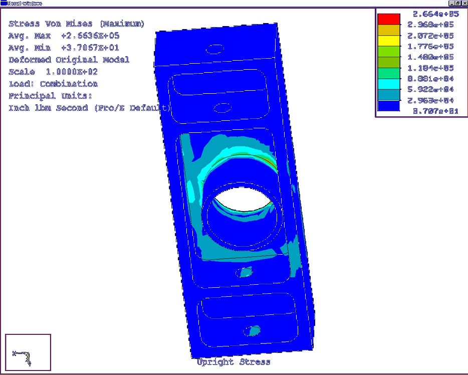
Figure 33. Front left upright under 1.5G right turn cornering and 1.2G braking.
After the analysis detailed on the preceding pages, the authors manufactured one front suspension prototype and one rear suspension prototype, each of which includes, an upright/hub assembly the control arms and mounting brackets for control arms and dampers. The rear suspension includes a track rod. Purchased items include rod ends (spherical ball bearings with a shank to thread into the control arms), control arm tubing adapters for the rod ends, rectangular tubing for the brackets, nuts, bolts, washers and dampers. Appropriate wheels were sourced and purchased earlier to determine the packaging requirements for the suspensions. The authors are working on finding a good deal for the springs. Details on items purchased are given in the Appendix on page
*.Because the points specified with Reynard Kinematics are endpoints about which suspension members rotate, the true control arm lengths and some angles cannot be derived straight from Reynard Kinematics. Instead, detailed trigonometry and consideration of the dimensions of each part is needed to determine true lengths and angles for cutting. A Microsoft Excel sheet has been created to convert the Reynard Kinematics’ virtual points into actual workable dimensions in inches and is shown in the Appendix on page
*.The uprights are machined (CNC) out of 6061-T6 (verify). Aluminum was chosen for its greater strength to weight ratio to reduce unsprung weight. Also, because these uprights are only a prototype (the brake and wheel attachments have yet to be designed), making the uprights out of aluminum is faster than structurally comparable pieces of steel. The front and rear uprights are shown in Figure 34. The front upright is the one on the right (no attachment for toe control track rod).
The control arms are made from 4130N chromoly steel tubing with an outside diameter of 0.75 in and a wall thickness of 0.58 in. Calculations performed later show that these offer a large factor of safety for all expected loads. The brackets are of the same grade steel, but made from rectangular tubing with a 1.5 in by 1.0 in cross section and a wall thickness of 0.65 in. The control arm adapters are also the same chromoly but polished and machined by the supplier.
Heavy duty shank rod ends are used with 0.4375 in threaded shanks and 0.375 bolts. The authors have worked with the rod end supplier to ensure that these rod ends are strong enough for our expected loads. Due to the incline of the upper control arms for the rear suspension system, high misalignment rod ends are used. The other components use regular rod ends as they do not need angles higher than the permissible angles of regular rod ends.
High quality airframe/aircraft bolts are used, together with corresponding washers and locknuts and jamnuts. Bolts for all rod ends are 0.375 in, with unthreaded portions for load surfaces. Bolts for the dampers are 0.5 in as required by the damper eyelets.
Progress Summary and Future Work
The authors feel that the suspension design and prototypes to date reflect the four main Princeton Formula SAE philosophies for its first car. The choice of an independent double A-arm system using outboard springs and dampers was seen as the best compromise of simplicity with adjustability. Furthermore, this system is certainly upgradable, such as by converting to an inboard system and by adding anti-roll bars. In making use of parametric software, the authors are happy with the kinematics, dynamics and strength of the suspension prototypes. However, some items require further validation and consideration, and these are listed below.
For the spring semester, the authors plan on creating a complete vehicle control package for the Princeton Formula SAE car, which includes designing the brake and steering systems. However, some suspension issues need to be resolved. First, although a front anti-roll bar rate has been specified from dynamic calculations, its packaging and manufacturing details will be finalized. The front suspension kinematics deserve another look to see if the roll center migration under roll can be reduced. Further analysis has to be done to ensure that the rear damper being mounted on the lower control arm itself is structurally sound. If not, a web can be made near the mounting area for increased strength. With the brake and steering systems specified, uprights that include mounting points for the brake caliper, spindle and other hardware need to be redesigned. The authors will also look into a less theoretical and more realistic method of analyzing vehicle dynamics, such as considering road inputs and the role of the frame and engine in affecting the dynamics, and making use of CarSim Educational.
Adams, Herb. Chassis Engineering: Chassis Design, Building & Tuning for High Performance Handling. Los Angeles: HP Books, 1993.
Aird, Forbes. Race Car Chassis: Design and Construction. Osceola: Motorbooks International, 1997.
Alexander, Don. Performance Handling: How to Make your Car Handle: Techniques for the 1990s. Osceola: Motorbooks International, 1997.
Carter, Campbell D., Cindy B. Sherman, and Ronald D. Matthews. "Design of a Formula SAE Race Car: Vehicle Dynamics and Performance." SAE Paper 821092, 1982.
Formula SAE 1999 brochure.
Gillespie, Thomas D. Fundamentals of Vehicle Dynamics. Warrendale: SAE, 1992.
Lopez, Carl, and Danny Sullivan. Going Faster: Mastering the Art of Race Driving: Cambridge: Bentley, 1998.
Milliken, William F., and Douglas L. Milliken. Race Car Vehicle Dynamics. Warrendale: SAE International, 1995.
Smith, Carroll. Carroll Smith’s Engineer in Your Pocket: A Practical Guide to Tuning the Race Car Chassis and Suspension. 1998.
Staniforth, Allan. Competition Car Suspension Design, Construction, Tuning. 3rd ed. Someset: Haynes, 1999.
Staniforth, Allan. Race and Rally Car Source Book: The Guide to Building or Modifying a Competition Car. 4th ed. Somerset: Haynes, 1997.
Gaffney, Edmund F. III, and Anthony R. Salinas. "Introduction to Formula SAE Suspension and Frame Design." SAE Paper 971584, 1997.
Goodyear Tire & Rubber Company. Tire Data for Formula SAE Program. Akron: Goodyear Technical Center.
Woods, David E, and Badih A. Jawad. "Numerical Design of Racecar Suspension Parameters." SAE Paper 1999-01-2257, 1999.
Various catalogs and brochures.
Definitions (Suspension Kinematics)
The definitions here are in the same order in which they appear in the discussion of suspension kinematics on page
*.Bump, jounce or compression is used to describe the motion of the wheel and tire when they move upward with respect to the vehicle body.
Rebound, droop or extension is used to describe the motion of the wheel and tire when they move downward with respect to the vehicle body.
Wheel travel is not an official term, but in this paper, it is used to mean the bump and rebound motions of the wheel, tire and related suspension components.
Camber is the angle by which a tire deviates from being perpendicular to the ground when viewed from the front or rear of the vehicle, as shown in Figure 35. The camber is negative if the angle between the inboard side of the tire and the ground is acute and positive if this angle is obtuse.
Toe is the angle at which the tires point toward or away from each other from the top view of the car. Toe-in (or positive toe) is when the tires point toward each other in the direction of travel. Toe-out (or negative toe) is when the tires point away from each other in the direction of travel.
Bump steer is the change in toe with wheel travel, and it occurs because the tie rod can be of a different length or oriented differently with respect to the rest of the control arms. For example, if the tie rod is mounted below the wheel centerline, and its radius of curvature is shorter than the radius of curvature of the other control arms, the tire will toe-out on both bump and rebound. This is shown in Figure 36.

Figure 36. Tie rod too short causes toe changes (bump steer). (Milliken)
If, on the other hand, the radius of curvature is correct but the end of the tie rod is mounted too high on the upright side of the suspension or too low on the side of the steering rack, the tire will toe-out on bump and toe-in on rebound. This causes both wheels to steer out of the turn and can be used as an understeer effect.
,
Figure 37. Tie rod in the wrong vertical location causes toe changes (bump steer). (Milliken)

Figure 38. Suspension and steering geometry. (Milliken)
The steering axis is the line about which the front wheels turn relative to the car when steered. The dotted lines in Figure 38 above shows the steering axis in both the front view and side view. In practice, the steering axis is usually not perfectly vertical and perpendicular to the ground, for reasons to be discussed under Caster, Kingpin Inclination and Trail.
Trail is the fore/aft distance between the contact patch of a tire and where the steering axis intersects the ground. Usually, the steering axis intersects the ground at a point forward of the contact patch of the tire. Figure 38 shows the physical interpretation of mechanical trail. Because the tire rubber deforms, the real contact patch of a tire is to the rear of what Figure 38 indicates. This additional trail, the pneumatic trail, adds to the mechanical trail to form the total trail.
Caster is the angle that the steering axis deviates from vertical in the side view of a vehicle, as shown in Figure 38. If the lower ball joint is forward of the upper ball joint, the caster angle is positive. Caster is important when the wheels are steered, so it has minimal effect on the rear suspension system.
Scrub radius is the cross-car (left-right) distance between the contact patch of a tire and where the steering axis intersects the ground. The scrub radius is considered positive if the tire contact patch is farther outboard than where the steering axis intersects the ground.
The kingpin inclination (also referred to as the steering axis lateral inclination) is the angle that the steering axis deviates from vertical in the front or rear view of a vehicle. See Figure 38.
Definitions (Suspension Dynamics)
The order of the definitions follow the order of the discussion in the main text.
Slip angle
The slip angle is the angle between the direction of tire heading and the actual direction of travel of the wheel. If a lateral load exists such that the contact patch points in a slightly different direction from the rest of the tire, a slip angle exists. Another way of picturing slip angle is by imagining the angle between the wheel plane (which defines the direction of the heading) and the contact patch’s direction of travel.
Understeer is perceived by the driver as the tendency of a car being unable to make a turn that is as tight as the driver inputs by turning the steering wheel. Technically, understeer is defined by slip angles, steering wheel angle gradients and Ackermann steer angle gradients, among other parameters.
Mild understeer usually goes unnoticed by the inexperienced drivers who simply turn the steering wheel more, although the car usually feels like it’s running wide and that more steering lock is required.Oversteer is easily perceived by the driver as the rear tires losing traction and that the rear end of the vehicle is about to initiate a spin.
A neutral attitude is one that is characterized by neither understeer nor oversteer.
The spring rate is simply the constant of proportionality between spring displacement from equilibrium and its restoring force. Despite the definition above, the spring rate may not be constant. Manufacturing processes and the spring geometry may be tailored to provide a progressive spring (one whose rate increases with displacement from equilibrium) or a digressive spring (one whose rate decreases with displacement from equilibrium).
The tire rate is the vertical force per unit of vertical displacement of the tire. A tire can be modeled as a spring that deflects under vertical load. Using this model, the tire rate is the spring rate of the tire.
The wheel rate is the vertical force per unit of vertical displacement at the wheel centerline relative to the fixed frame.
The ride rate is the vertical force per unit of vertical displacement of the tire contact patch relative to the fixed frame. The value of the ride rate is the effective rate using the wheel rate and the tire rate in series. Thus, for any tire that is not infinitely stiff, the ride rate is always less than the wheel rate. In most motorsports (Formula 1 is a notable exception), the tire rate is several orders of magnitude greater than the wheel rate, so the ride rate can be approximated as the wheel rate.
The ride frequency is the ride rate, normalized by the mass of the sprung corner weight and expressed in Hertz or cycles per minute. Because the ride frequency is scaled by the sprung mass, its value is applicable across different vehicle types regardless of the vehicle weight. Also, the static wheel deflection per unit of vertical acceleration can be mapped directly with the ride frequency.
The motion ratio is a dimensionless number that compares the motion of two items. In this report, the motion ratio is the ratio of the spring/damper movement per unit of wheel travel.
Load transfer refers to the phenomenon where the acceleration of the vehicle body causes a change in the vertical (normal) forces experienced by the tires from what they were when the vehicle was stationary or not accelerating.
An anti-roll bar is usually a torsion bar that couples the left and right wheels on a car with independent suspension such that, when only one wheel tries to bump or rebound independently of the other, the anti-roll bar is placed in torsion. The anti-roll bar acts as a spring that resists independent motion of the wheels. A true anti-roll bar does not have any dynamic effect when both the left and right wheels try to move together such as during brake induced body pitching.
Vehicle Dynamics Calculations Spreadsheet
Figure 39. Spreadsheet showing the calculation of vehicle dynamics parameters.
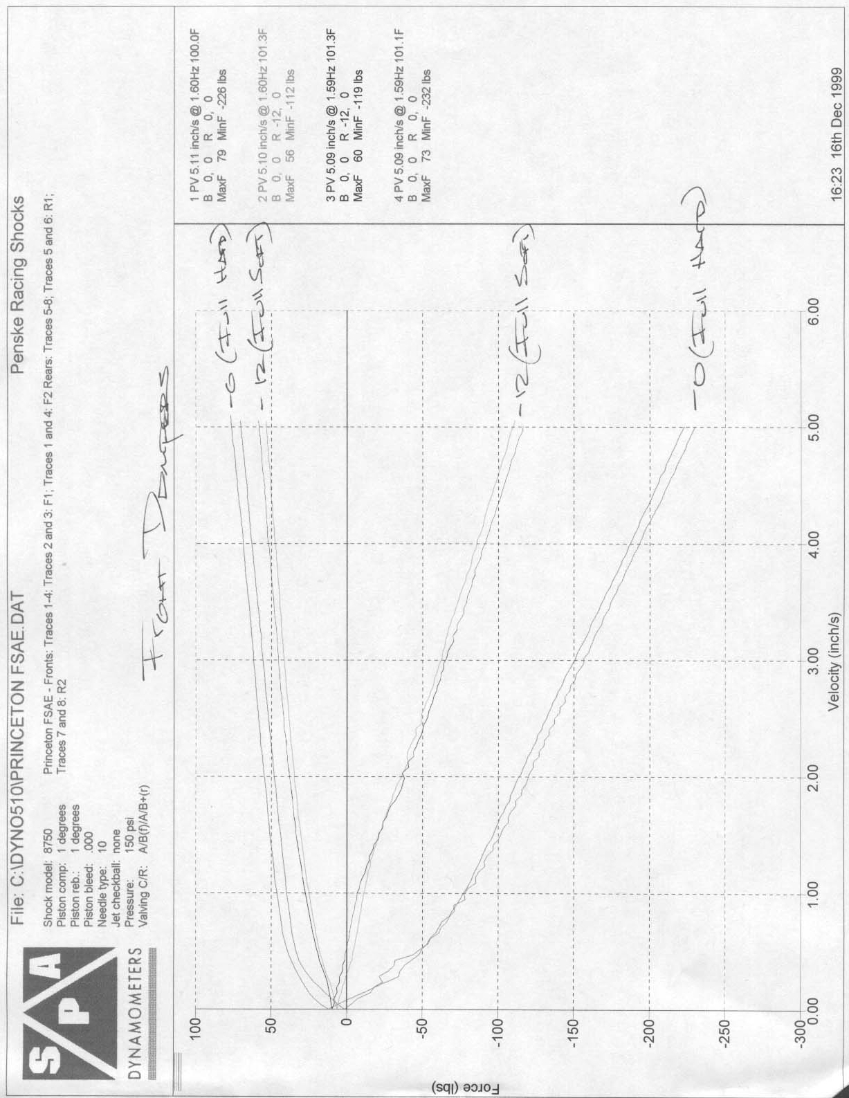
Figure 40. Front damper dyno plot.
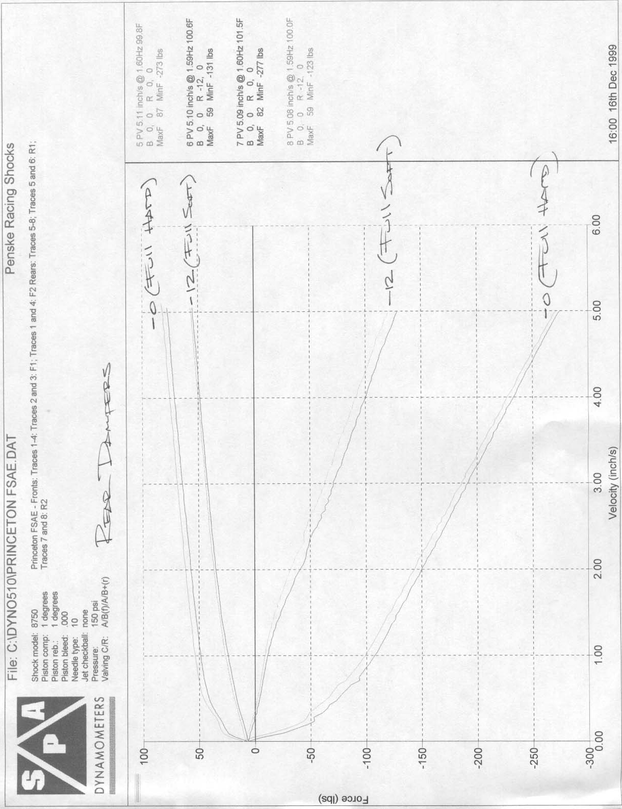
Figure 41. Rear damper dyno plot.
Front Suspension
Figure 42. Front suspension A-arm dimensions.
Rear Suspension
Figure 43. Rear suspension A-arm dimensions.
Front Suspension Load Calculations
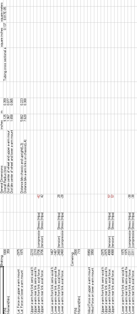
Figure 44. Front suspension load calculations.
Rear Suspension Load Calculations
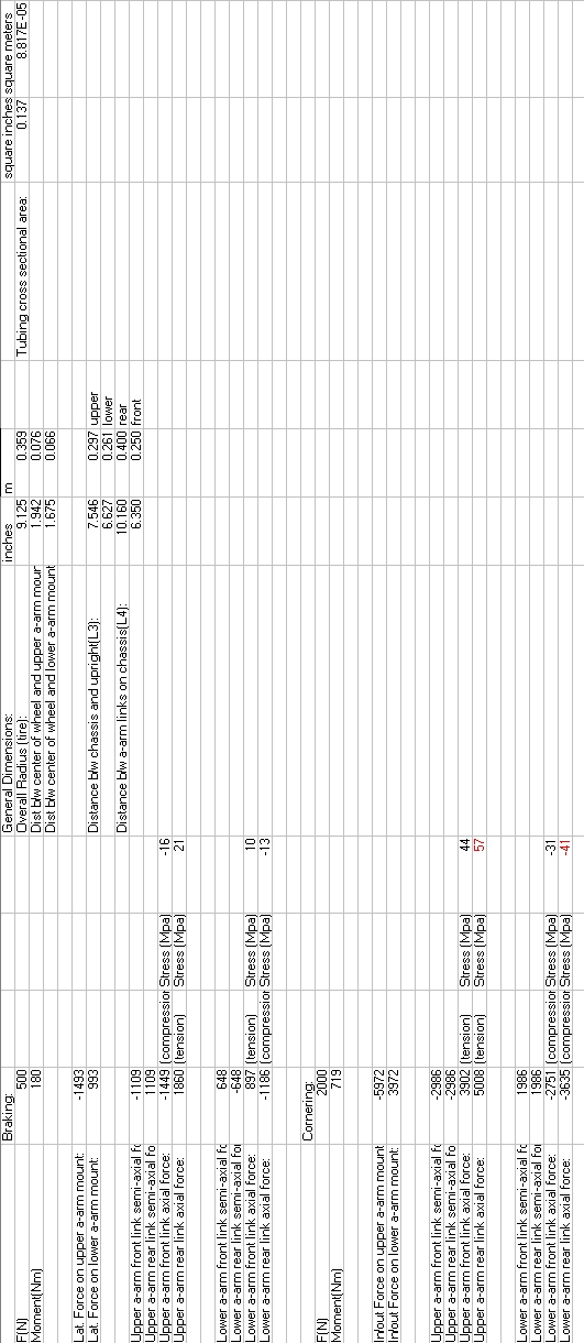
Figure 45. Rear suspension load calculations.
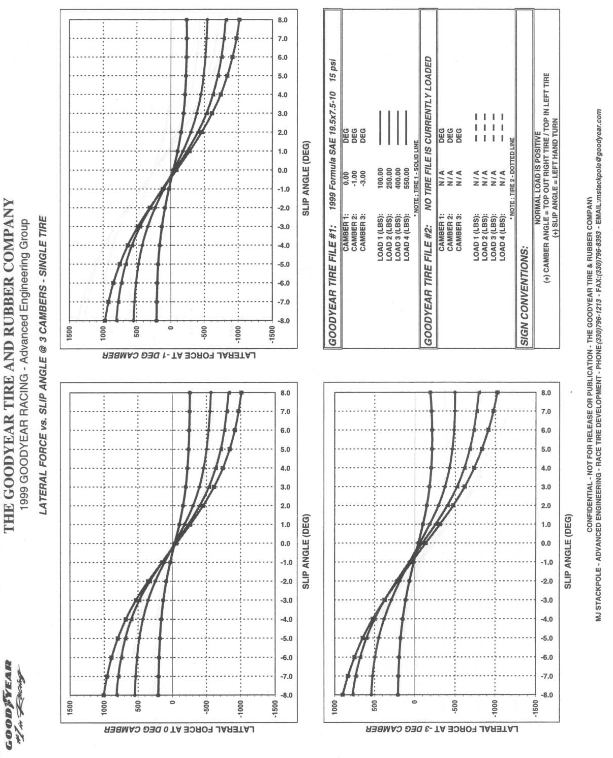
Purchased Parts, Suppliers and Prices for Fall 1999
|
Part |
Supplier/Vendor |
Cost |
|
4 wheels |
Keizer Aluminum Wheels |
$321.00 |
|
24 ft. Control arm tubing 28 Control arm tubing adapters |
Chassis Shop Performance Products |
$138.53 |
|
4 ft. Frame attachment rectangular tubing |
Chassis Shop Performance Products |
$48.50 |
|
30 Airframe bolts |
Pegasus Auto Racing Supplies |
$38.94 |
|
30 Nylock Nuts 30 Jamnuts 200 Washers |
TrueChoice Motorsports |
$30.70 |
|
4 Dampers |
Penske Racing Shocks |
$1,023.00 |
|
4 ft. Frame attachment rectangular tubing |
Chassis Shop Performance Products |
$48.50 |
|
30 Jamnuts |
TrueChoice Motorsports |
$23.40 |
|
10 Airframe bolts 5 Nylock nuts 100 Washers |
TrueChoice Motorsports |
$39.15 |
|
9 Regular rod ends 4 High misalignment rod ends |
Aurora Bearing Company |
$177.67 |
|
Jamnuts refund |
TrueChoice Motorsports |
-$11 |
|
Vehicle Control Division Semester Total |
$1878.39 |